Language models accurately infer correlations between psychological items and scales from text alone

Here, we apply the pre-trained model and our fine-tuned model to data not used for training, a holdout. The holdout sample was collected by Bainbridge et al. 2022.

knitr::opts_chunk$set(echo = TRUE, error = T, message = F, warning = F)

# Libraries and Settings

# Libs ---------------------------
library(knitr)
library(tidyverse)
library(arrow)
library(glue)
library(psych)
library(lavaan)
library(ggplot2)
library(plotly)
library(gridExtra)
library(broom)
library(broom.mixed)
library(brms)
library(tidybayes)
library(cmdstanr)
library(cowplot)

options(mc.cores = parallel::detectCores(), 
        brms.backend = "cmdstanr", 
        brms.file_refit = "on_change")


model_name = "ItemSimilarityTraining-20240502-trial12"
#model_name = "item-similarity-20231018-122504"
pretrained_model_name = "all-mpnet-base-v2"

data_path = glue("./")
pretrained_data_path = glue("./")

set.seed(42)


holdout <- arrow::read_feather(file = file.path(data_path, glue("data/intermediate/{model_name}.raw.osf-bainbridge-2021-s2-0.item_correlations.feather")))

pt_holdout <- arrow::read_feather(file = file.path(data_path, glue("data/intermediate/{pretrained_model_name}.raw.osf-bainbridge-2021-s2-0.item_correlations.feather")))

holdout_mapping_data = arrow::read_feather(
  file = file.path(data_path, glue("{model_name}.raw.osf-bainbridge-2021-s2-0.mapping2.feather"))
) %>%
  rename(scale_0 = scale0,
         scale_1 = scale1)

holdout_human_data = arrow::read_feather(
  file = file.path(data_path, glue("{model_name}.raw.osf-bainbridge-2021-s2-0.human.feather"))
)

holdout_scales <- arrow::read_feather(file.path(data_path, glue("{model_name}.raw.osf-bainbridge-2021-s2-0.scales.feather"))
)

N <- holdout_human_data %>% summarise_all(~ sum(!is.na(.))) %>% min()
total_N <- nrow(holdout_human_data)

The Bainbridge data was collected on N=493 respondents. The item with the most missing values still had n=480.

Synthetic inter-item correlations

holdout_llm <- holdout %>%
  left_join(holdout_mapping_data %>% select(variable_1 = variable, InstrumentA = instrument, ScaleA = scale_0, SubscaleA = scale_1)) %>%
  left_join(holdout_mapping_data %>% select(variable_2 = variable, InstrumentB = instrument, ScaleB = scale_0, SubscaleB = scale_1))

pt_holdout_llm <- pt_holdout %>%
  left_join(holdout_mapping_data %>% select(variable_1 = variable, InstrumentA = instrument, ScaleA = scale_0, SubscaleA = scale_1)) %>%
  left_join(holdout_mapping_data %>% select(variable_2 = variable, InstrumentB = instrument, ScaleB = scale_0, SubscaleB = scale_1))

Accuracy

se2 <- mean(holdout_llm$empirical_r_se^2)

r <- broom::tidy(cor.test(holdout_llm$empirical_r, holdout_llm$synthetic_r))
pt_r <- broom::tidy(cor.test(pt_holdout_llm$empirical_r, pt_holdout_llm$synthetic_r))

model <- paste0('
  # Latent variables
  PearsonLatent =~ 1*empirical_r

  # Fixing error variances based on known standard errors
  empirical_r ~~ ',se2,'*empirical_r

  # Relationship between latent variables
  PearsonLatent ~~ synthetic_r
')

fit <- sem(model, data = holdout_llm)
pt_fit <- sem(model, data = pt_holdout_llm)

m_synth_r_items <- brm(
  bf(empirical_r | mi(empirical_r_se) ~ synthetic_r + (1|mm(variable_1, variable_2)),
     sigma ~ s(synthetic_r)), data = holdout_llm, 
  file = "ignore/m_synth_r_items_lm")

sd_synth <- sd(m_synth_r_items$data$synthetic_r)

newdata <- m_synth_r_items$data %>% select(empirical_r, synthetic_r, empirical_r_se)
epreds <- epred_draws(newdata = newdata, obj = m_synth_r_items, re_formula = NA, ndraws = 200)
preds <- predicted_draws(newdata = newdata, obj = m_synth_r_items, re_formula = NA, ndraws = 200)
epred_preds <- epreds %>% left_join(preds)
by_draw <- epred_preds %>% group_by(.draw) %>% 
  summarise(mae = mean(abs(.epred - .prediction)),
            .epred = var(.epred),
            .prediction = var(.prediction),
            sigma = sqrt(.prediction - .epred),
            latent_r = sqrt(.epred/.prediction))
rm(epred_preds)

accuracy_bayes_items <- by_draw %>% mean_hdci(latent_r)

bind_rows(
  pt_r %>% 
    mutate(model = "pre-trained", kind = "manifest") %>% 
    select(model, kind, accuracy = estimate, conf.low, conf.high),
  standardizedsolution(pt_fit) %>% 
    filter(lhs == "PearsonLatent", rhs ==  "synthetic_r") %>% 
    mutate(model = "pre-trained", kind = "latent outcome (SEM)") %>% 
    select(model, kind, accuracy = est.std, 
           conf.low = ci.lower, conf.high = ci.upper),
  r %>% 
    mutate(model = "fine-tuned", kind = "manifest") %>% 
    select(model, kind, accuracy = estimate, conf.low, conf.high),
  standardizedsolution(fit) %>% 
    filter(lhs == "PearsonLatent", rhs ==  "synthetic_r") %>% 
    mutate(model = "fine-tuned", kind = "latent outcome (SEM)") %>% 
    select(model, kind, accuracy = est.std, 
           conf.low = ci.lower, conf.high = ci.upper),
  accuracy_bayes_items %>% 
    mutate(model = "fine-tuned", kind = "latent outcome (Bayesian EIV)") %>% 
    select(model, kind, accuracy = latent_r, conf.low = .lower, conf.high = .upper)
) %>% 
  knitr::kable(digits = 2)

model	kind	accuracy	conf.low	conf.high
pre-trained	manifest	0.19	0.18	0.19
pre-trained	latent outcome (SEM)	0.19	0.19	0.20
fine-tuned	manifest	0.67	0.67	0.68
fine-tuned	latent outcome (SEM)	0.70	0.70	0.70
fine-tuned	latent outcome (Bayesian EIV)	0.71	0.70	0.72

Prediction error plot according to synthetic estimate

m_synth_r_items

##  Family: gaussian 
##   Links: mu = identity; sigma = log 
## Formula: empirical_r | mi(empirical_r_se) ~ synthetic_r + (1 | mm(variable_1, variable_2)) 
##          sigma ~ s(synthetic_r)
##    Data: holdout_llm (Number of observations: 87153) 
##   Draws: 4 chains, each with iter = 2000; warmup = 1000; thin = 1;
##          total post-warmup draws = 4000
## 
## Smoothing Spline Hyperparameters:
##                           Estimate Est.Error l-95% CI u-95% CI Rhat Bulk_ESS
## sds(sigma_ssynthetic_r_1)     0.64      0.24     0.30     1.25 1.00     1402
##                           Tail_ESS
## sds(sigma_ssynthetic_r_1)     2008
## 
## Multilevel Hyperparameters:
## ~mmvariable_1variable_2 (Number of levels: 418) 
##               Estimate Est.Error l-95% CI u-95% CI Rhat Bulk_ESS Tail_ESS
## sd(Intercept)     0.03      0.00     0.03     0.03 1.00      889     1498
## 
## Regression Coefficients:
##                      Estimate Est.Error l-95% CI u-95% CI Rhat Bulk_ESS
## Intercept               -0.01      0.00    -0.01    -0.00 1.01      636
## sigma_Intercept         -2.20      0.00    -2.21    -2.20 1.00     5202
## synthetic_r              0.79      0.00     0.78     0.80 1.00     5610
## sigma_ssynthetic_r_1    -1.50      0.82    -3.19    -0.03 1.00     2219
##                      Tail_ESS
## Intercept                1307
## sigma_Intercept          3543
## synthetic_r              3282
## sigma_ssynthetic_r_1     2824
## 
## Draws were sampled using sample(hmc). For each parameter, Bulk_ESS
## and Tail_ESS are effective sample size measures, and Rhat is the potential
## scale reduction factor on split chains (at convergence, Rhat = 1).

pred <- conditional_effects(m_synth_r_items, method = "predict")
kable(rmse_items <- by_draw %>% mean_hdci(sigma), caption = "Average prediction error (RMSE)", digits = 2)

Average prediction error (RMSE)

sigma	.lower	.upper	.width	.point	.interval
0.11	0.11	0.11	0.95	mean	hdci

kable(mae_items <- by_draw %>% mean_hdci(mae), caption = "Average prediction error (MAE)", digits = 2)

Average prediction error (MAE)

mae	.lower	.upper	.width	.point	.interval
0.09	0.09	0.09	0.95	mean	hdci

plot_prediction_error_items <- plot(conditional_effects(m_synth_r_items, dpar = "sigma"), plot = F)[[1]] + 
  theme_bw() + 
  xlab("Synthetic inter-item correlation") + 
  ylab("Prediction error (sigma)") +
  geom_smooth(stat = "identity", color = "#a48500", fill = "#EDC951")

plot_prediction_error_items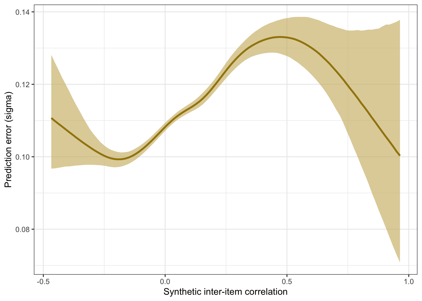

Scatter plot

ggplot(holdout_llm, aes(synthetic_r, empirical_r, 
              ymin = empirical_r - empirical_r_se,
              ymax = empirical_r + empirical_r_se)) + 
  geom_abline(linetype = "dashed") +
  geom_point(color = "#00A0B0", alpha = 0.1, size = 1) +
  geom_smooth(aes(
    x = synthetic_r,
    y = estimate__,
    ymin = lower__,
    ymax = upper__,
  ), stat = "identity", 
  color = "#a48500",
  fill = "#EDC951",
  data = as.data.frame(pred$synthetic_r)) +
  xlab("Synthetic inter-item correlation") + 
  ylab("Empirical inter-item correlation") +
  theme_bw() +
  coord_fixed(xlim = c(-1,1), ylim = c(-1,1)) -> plot_items
plot_items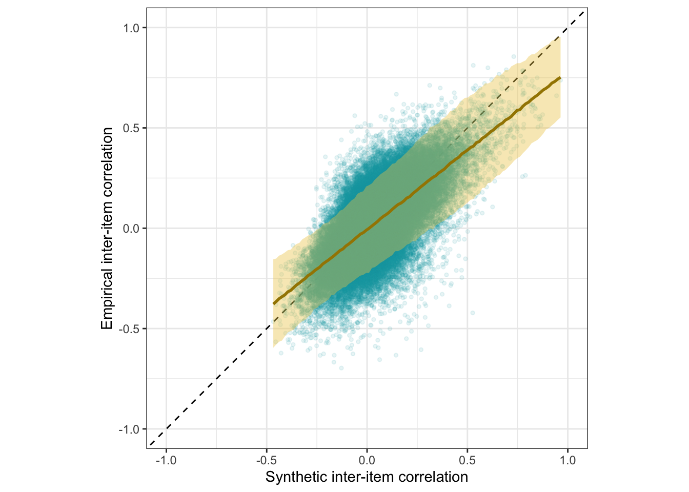

Interactive plot

This plot shows only 2000 randomly selected item pairs to conserve memory. A full interactive plot exists, but may react slowly.

item_pair_table <- holdout_llm %>% 
   left_join(holdout_mapping_data %>% select(variable_1 = variable,
                                             item_text_1 = item_text)) %>% 
   left_join(holdout_mapping_data %>% select(variable_2 = variable,
                                             item_text_2 = item_text))

# item_pair_table %>% filter(str_length(item_text_1) < 30, str_length(item_text_2) < 30) %>% 
#   left_join(pt_holdout_llm %>% rename(synthetic_r_pt = synthetic_r)) %>% 
#   select(item_text_1, item_text_2, empirical_r, synthetic_r, synthetic_r_pt) %>% View()
rio::export(item_pair_table, "ignore/item_pair_table.feather")

(item_pair_table %>% 
  mutate(synthetic_r = round(synthetic_r, 2),
         empirical_r = round(empirical_r, 2),
         items = str_replace_all(str_c(item_text_1, "\n", item_text_2),
                                  "_+", " ")) %>% 
    sample_n(2000) %>%
ggplot(., aes(synthetic_r, empirical_r, 
              # ymin = empirical_r - empirical_r_se, 
              # ymax = empirical_r + empirical_r_se, 
              label = items)) + 
  geom_abline(linetype = "dashed") +
  geom_point(color = "#00A0B0", alpha = 0.3, size = 1) +
  xlab("Synthetic inter-item correlation") + 
  ylab("Empirical inter-item correlation") +
  theme_bw() +
  coord_fixed(xlim = c(-1,1), ylim = c(-1,1))) %>% 
  ggplotly()

item_pair_table <- item_pair_table %>% 
  mutate(empirical_r = sprintf("%.2f±%.3f", empirical_r,
                                 empirical_r_se),
           synthetic_r = sprintf("%.2f", synthetic_r)) %>% 
  select(item_text_1, item_text_2, empirical_r, synthetic_r)
rio::export(item_pair_table, "item_pair_table.xlsx")

Robustness checks

Comparing spline and polynomial models for heteroscedasticity

m_synth_r_items_poly <- brm(
  bf(empirical_r | mi(empirical_r_se) ~ synthetic_r + (1|mm(variable_1, variable_2)),
     sigma ~ poly(synthetic_r, degree = 3)), data = holdout_llm, 
  file = "ignore/m_synth_r_items_lm_poly")

newdata <- m_synth_r_items_poly$data %>% select(empirical_r, synthetic_r, empirical_r_se)
epreds <- epred_draws(newdata = newdata, obj = m_synth_r_items_poly, re_formula = NA, ndraws = 200)
preds <- predicted_draws(newdata = newdata, obj = m_synth_r_items_poly, re_formula = NA, ndraws = 200)
epred_preds <- epreds %>% left_join(preds)
by_draw <- epred_preds %>% group_by(.draw) %>% 
  summarise(.epred = var(.epred),
            .prediction = var(.prediction),
            sigma = sqrt(.prediction - .epred),
            latent_r = sqrt(.epred/.prediction))

accuracy_bayes_items_poly <- by_draw %>% mean_hdci(latent_r)

bind_rows(
  accuracy_bayes_items %>% 
    mutate(model = "spline", kind = "latent outcome (Bayesian EIV)") %>% 
    select(model, kind, accuracy = latent_r, conf.low = .lower, conf.high = .upper),
  accuracy_bayes_items_poly %>% 
    mutate(model = "polynomial", kind = "latent outcome (Bayesian EIV)") %>% 
    select(model, kind, accuracy = latent_r, conf.low = .lower, conf.high = .upper)
) %>% 
  knitr::kable(digits = 2, caption = "Comparing spline and polynomial models for item correlations")

Comparing spline and polynomial models for item correlations

model	kind	accuracy	conf.low	conf.high
spline	latent outcome (Bayesian EIV)	0.71	0.7	0.72
polynomial	latent outcome (Bayesian EIV)	0.71	0.7	0.72

plot_prediction_error_items_poly <- plot(conditional_effects(m_synth_r_items_poly, dpar = "sigma"), plot = F)[[1]] + 
  theme_bw() + 
  xlab("Synthetic inter-item correlation") + 
  ylab("Prediction error (sigma)") +
  geom_smooth(stat = "identity", color = "#a48500", fill = "#EDC951")

plot_prediction_error_items_poly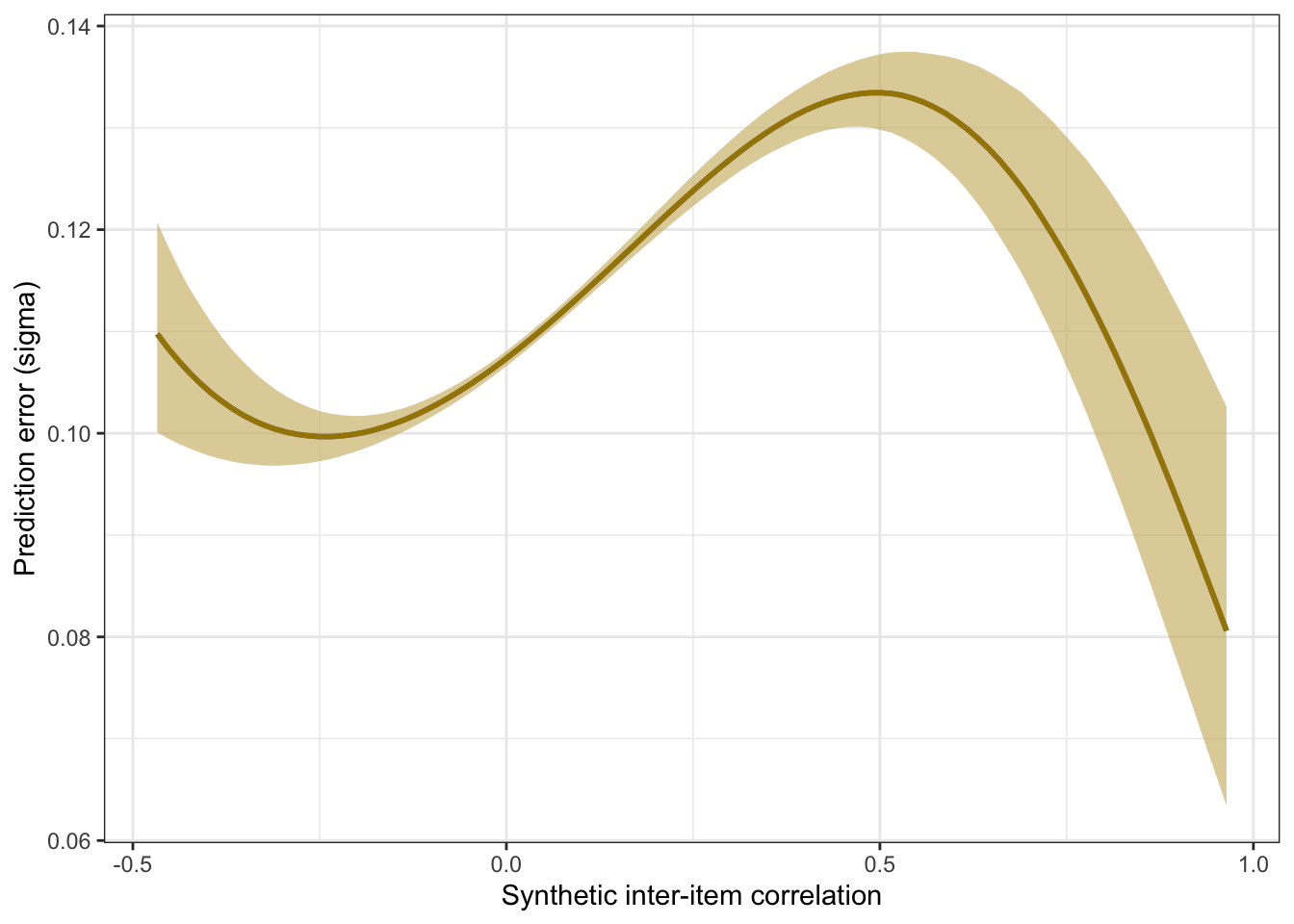

Is the accuracy lower within/across scales and instruments?

holdout_llm %>% 
  mutate(same_instrument = if_else(InstrumentA == InstrumentB, 1, 0,0),
         same_scale = if_else(ScaleA == ScaleB, 1,0,0),
         same_subscale = if_else(same_scale & SubscaleA == SubscaleB, 1,0,0)) %>% 
  group_by(same_scale, same_instrument, same_subscale) %>% 
  summarise(broom::tidy(cor.test(synthetic_r, empirical_r)), sd_emp_r = sd(empirical_r), n = n()) %>% 
  select(same_instrument, same_scale, same_subscale, r = estimate, conf.low, conf.high, n, sd_emp_r) %>% 
  arrange(same_instrument, same_scale, same_subscale) %>% 
  kable()

same_instrument	same_scale	same_subscale	r	conf.low	conf.high	n	sd_emp_r
0	0	0	0.6525977	0.6484796	0.6566776	75364	0.1537790
0	1	0	0.8269917	0.8095247	0.8429959	1376	0.2801202
0	1	1	0.8269181	0.7293619	0.8915144	64	0.4934840
1	0	0	0.6005392	0.5855629	0.6151056	7200	0.1365890
1	1	0	0.7571886	0.7404990	0.7729447	2662	0.2582187
1	1	1	0.8372433	0.8085383	0.8619731	487	0.3847884

Is the accuracy lower outside classic Big Five?

holdout_llm %>% 
  mutate(big_five = case_when(
    str_detect(InstrumentA, "(Personality|Big Five)") & str_detect(InstrumentB, "(Personality|Big Five)") ~ "both",
    str_detect(InstrumentA, "(Personality|Big Five)") | str_detect(InstrumentB, "(Personality|Big Five)") ~ "either",
    TRUE ~ "none"
         )) %>% 
  group_by(big_five) %>% 
  summarise(broom::tidy(cor.test(synthetic_r, empirical_r)), sd_emp_r = sd(empirical_r), n = n()) %>% 
  select(big_five, r = estimate, conf.low, conf.high, n, sd_emp_r) %>% 
  arrange(big_five) %>% 
  kable()

big_five	r	conf.low	conf.high	n	sd_emp_r
both	0.7105135	0.7027822	0.7180770	16110	0.1754473
either	0.6618969	0.6565425	0.6671846	42840	0.1525947
none	0.6653591	0.6588041	0.6718132	28203	0.1697589

Is the accuracy lower for items that have low variance?

item_variances <- holdout_human_data %>% summarise_all(~ sd(., na.rm = T)) %>% 
  pivot_longer(everything(), names_to = "variable", values_to = "item_sd")

by_max_cov <- holdout_llm %>% 
  left_join(item_variances, by = c("variable_1" = "variable")) %>% 
  left_join(item_variances, by = c("variable_2" = "variable"), suffix = c("_1", "_2")) %>% 
  mutate(max_covariance = ceiling((item_sd_1 * item_sd_2)*10)/10)

rs_by_max_cov <- by_max_cov %>% 
  group_by(max_covariance) %>% 
  filter(n() > 3) %>% 
  summarise(broom::tidy(cor.test(synthetic_r, empirical_r)), sd_emp_r = sd(empirical_r), n = n()) %>% 
  select(max_covariance, r = estimate, conf.low, conf.high, n, sd_emp_r) %>% 
  arrange(max_covariance)

rs_by_max_cov%>% 
  kable()

max_covariance	r	conf.low	conf.high	n	sd_emp_r
0.5	0.8845860	0.6925673	0.9595392	16	0.0841287
0.6	0.5394056	0.4566420	0.6129128	319	0.1712504
0.7	0.5773367	0.5485306	0.6047739	2162	0.1591129
0.8	0.6331256	0.6192313	0.6466235	7355	0.1524384
0.9	0.6439129	0.6346448	0.6529958	15639	0.1496275
1.0	0.6333785	0.6255374	0.6410916	22779	0.1536605
1.1	0.6791602	0.6718518	0.6863364	21261	0.1657358
1.2	0.7290679	0.7206660	0.7372557	12257	0.1799820
1.3	0.7435976	0.7298785	0.7567179	4268	0.1774902
1.4	0.7194644	0.6869514	0.7491027	930	0.1587180
1.5	0.7077049	0.6188080	0.7787043	154	0.1447413
1.6	0.8896940	0.6452603	0.9688857	12	0.1835193

rs_by_max_cov %>% ggplot(aes(max_covariance, r, ymin = conf.low, ymax = conf.high)) +
  geom_pointrange()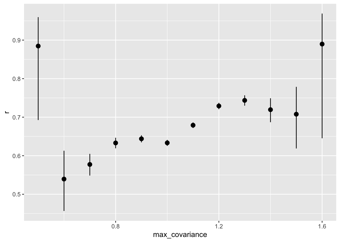

by_max_cov%>% 
  filter(max_covariance > .7) %>% 
  summarise(broom::tidy(cor.test(synthetic_r, empirical_r)), sd_emp_r = sd(empirical_r), n = n()) %>% 
  kable()

estimate	statistic	p.value	parameter	conf.low	conf.high	method	alternative	sd_emp_r	n
0.6758603	266.806	0	84654	0.6721843	0.6795029	Pearson’s product-moment correlation	two.sided	0.1624048	84656

holdout_llm %>% 
  left_join(item_variances, by = c("variable_1" = "variable")) %>% 
  left_join(item_variances, by = c("variable_2" = "variable"), suffix = c("_1", "_2")) %>% 
  mutate(max_covariance = ceiling((item_sd_1 * item_sd_2)*10)/10) %>% 
  filter(max_covariance > 1) %>% 
  summarise(broom::tidy(cor.test(synthetic_r, empirical_r)), sd_emp_r = sd(empirical_r), n = n()) %>% 
  select(r = estimate, conf.low, conf.high, n, sd_emp_r) %>% 
  knitr::kable()

r	conf.low	conf.high	n	sd_emp_r
0.7085118	0.7035267	0.7134273	38883	0.1726419

Averages

holdout_llm %>% summarise(
  mean(synthetic_r),
  mean(empirical_r),
  mean(abs(synthetic_r)),
  mean(abs(empirical_r)),
  prop_negative = sum(empirical_r < 0)/n(),
  prop_pos = sum(empirical_r > 0)/n(),
  `prop_below_-.10` = sum(empirical_r < -0.1)/n(),
  `prop_above_.10` = sum(empirical_r > 0.1)/n(),
) %>% kable(digits = 2, caption = "Average correlations")

Average correlations

mean(synthetic_r)	mean(empirical_r)	mean(abs(synthetic_r))	mean(abs(empirical_r))	prop_negative	prop_pos	prop_below_-.10	prop_above_.10
0.05	0.03	0.11	0.13	0.44	0.56	0.21	0.33

Is the accuracy lower for the pre-trained model?

ggplot(pt_holdout_llm, aes(synthetic_r, empirical_r, 
              ymin = empirical_r - empirical_r_se,
              ymax = empirical_r + empirical_r_se)) + 
  geom_abline(linetype = "dashed") +
  geom_point(color = "#00A0B0", alpha = 0.1, size = 1) +
  xlab("Synthetic inter-item correlation") + 
  ylab("Empirical inter-item correlation") +
  theme_bw() +
  coord_fixed(xlim = c(-1,1), ylim = c(-1,1)) -> pt_plot_items
pt_plot_items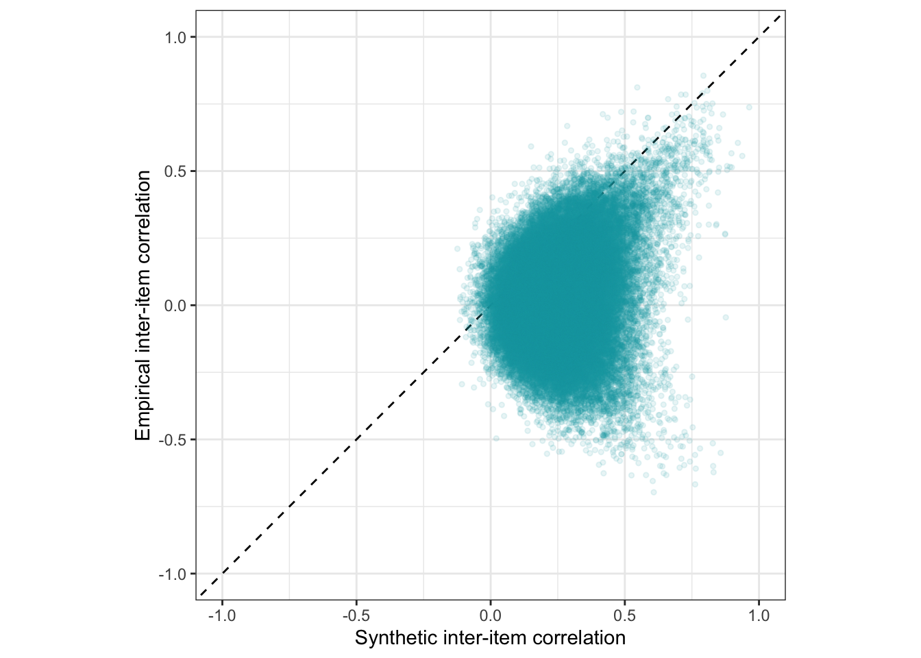

Full table of synthetic and empirical item pair correlations

Synthetic Reliabilities

scales <- read_rds(file = file.path(data_path, glue("data/intermediate/scales_with_alpha_se.rds")))


source("global_functions.R")

scales <- scales %>% filter(number_of_items >= 3)

Accuracy

se2 <- mean(scales$empirical_alpha_se^2)
r <- broom::tidy(cor.test(scales$empirical_alpha, scales$synthetic_alpha))
pt_r <- broom::tidy(cor.test(scales$empirical_alpha, scales$pt_synthetic_alpha))

model <- paste0('
  # Latent variables
  latent_real_rel =~ 1*empirical_alpha

  # Fixing error variances based on known standard errors
  empirical_alpha ~~ ',se2,'*empirical_alpha

  # Relationship between latent variables
  latent_real_rel ~~ synthetic_alpha
')

fit <- sem(model, data = scales)
pt_fit <- sem(model, data = scales %>% 
                select(empirical_alpha, synthetic_alpha = pt_synthetic_alpha))

m_lmsynth_rel_scales <- brm(
  bf(empirical_alpha | mi(empirical_alpha_se) ~ synthetic_alpha,
     sigma ~ s(synthetic_alpha)), data = scales, 
  file = "ignore/m_synth_rel_lm")

newdata <- m_lmsynth_rel_scales$data %>% select(empirical_alpha, synthetic_alpha, empirical_alpha_se)
epreds <- epred_draws(newdata = newdata, obj = m_lmsynth_rel_scales, re_formula = NA)
preds <- predicted_draws(newdata = newdata, obj = m_lmsynth_rel_scales, re_formula = NA)
epred_preds <- epreds %>% left_join(preds)
by_draw <- epred_preds %>% group_by(.draw) %>% 
  summarise(.epred = var(.epred),
            .prediction = var(.prediction),
            sigma = sqrt(.prediction - .epred),
            latent_r = sqrt(.epred/.prediction))

accuracy_bayes_rels <- by_draw %>% mean_hdci(latent_r)

bind_rows(
  pt_r %>% 
    mutate(model = "pre-trained", kind = "manifest") %>% 
    select(model, kind, accuracy = estimate, conf.low, conf.high),
  standardizedsolution(pt_fit) %>% 
    filter(lhs == "latent_real_rel", rhs ==  "synthetic_alpha") %>% 
    mutate(model = "pre-trained", kind = "latent outcome (SEM)") %>% 
    select(model, kind, accuracy = est.std, 
           conf.low = ci.lower, conf.high = ci.upper),
  r %>% 
    mutate(model = "fine-tuned", kind = "manifest") %>% 
    select(model, kind, accuracy = estimate, conf.low, conf.high),
  standardizedsolution(fit) %>% 
    filter(lhs == "latent_real_rel", rhs ==  "synthetic_alpha") %>% 
    mutate(model = "fine-tuned", kind = "latent outcome (SEM)") %>% 
    select(model, kind, accuracy = est.std, 
           conf.low = ci.lower, conf.high = ci.upper),
  accuracy_bayes_rels %>% 
    mutate(model = "fine-tuned", kind = "latent outcome (Bayesian EIV)") %>% 
    select(model, kind, accuracy = latent_r, conf.low = .lower, conf.high = .upper)
  ) %>% 
  knitr::kable(digits = 2)

model	kind	accuracy	conf.low	conf.high
pre-trained	manifest	0.38	0.28	0.48
pre-trained	latent outcome (SEM)	0.39	0.29	0.49
fine-tuned	manifest	0.89	0.86	0.91
fine-tuned	latent outcome (SEM)	0.90	0.87	0.92
fine-tuned	latent outcome (Bayesian EIV)	0.89	0.84	0.94

Prediction error plot according to synthetic estimate

m_lmsynth_rel_scales

##  Family: gaussian 
##   Links: mu = identity; sigma = log 
## Formula: empirical_alpha | mi(empirical_alpha_se) ~ synthetic_alpha 
##          sigma ~ s(synthetic_alpha)
##    Data: scales (Number of observations: 307) 
##   Draws: 4 chains, each with iter = 2000; warmup = 1000; thin = 1;
##          total post-warmup draws = 4000
## 
## Smoothing Spline Hyperparameters:
##                               Estimate Est.Error l-95% CI u-95% CI Rhat
## sds(sigma_ssynthetic_alpha_1)     3.35      1.43     1.32     6.94 1.00
##                               Bulk_ESS Tail_ESS
## sds(sigma_ssynthetic_alpha_1)      951      823
## 
## Regression Coefficients:
##                          Estimate Est.Error l-95% CI u-95% CI Rhat Bulk_ESS
## Intercept                    0.05      0.01     0.02     0.08 1.00     3077
## sigma_Intercept             -1.83      0.05    -1.92    -1.74 1.00     3731
## synthetic_alpha              0.96      0.02     0.92     1.00 1.00     3159
## sigma_ssynthetic_alpha_1    -1.56      5.57   -10.99    11.23 1.00     1181
##                          Tail_ESS
## Intercept                    3048
## sigma_Intercept              2992
## synthetic_alpha              3150
## sigma_ssynthetic_alpha_1      934
## 
## Draws were sampled using sample(hmc). For each parameter, Bulk_ESS
## and Tail_ESS are effective sample size measures, and Rhat is the potential
## scale reduction factor on split chains (at convergence, Rhat = 1).

pred <- conditional_effects(m_lmsynth_rel_scales, method = "predict")
kable(rmse_alpha <- by_draw %>% mean_hdci(sigma), caption = "Average prediction error (RMSE)", digits = 2)

Average prediction error (RMSE)

sigma	.lower	.upper	.width	.point	.interval
0.2	0.13	0.25	0.95	mean	hdci

plot_prediction_error_alpha <- plot(conditional_effects(m_lmsynth_rel_scales, dpar = "sigma"), plot = F)[[1]] + 
  theme_bw() + 
  geom_smooth(stat = "identity", color = "#a48500", fill = "#EDC951") + 
  xlab("Synthetic Cronbach's alpha") + 
  ylab("Prediction error (sigma)") +
  coord_cartesian(xlim = c(-1, 1), ylim = c(0, 0.35))
plot_prediction_error_alpha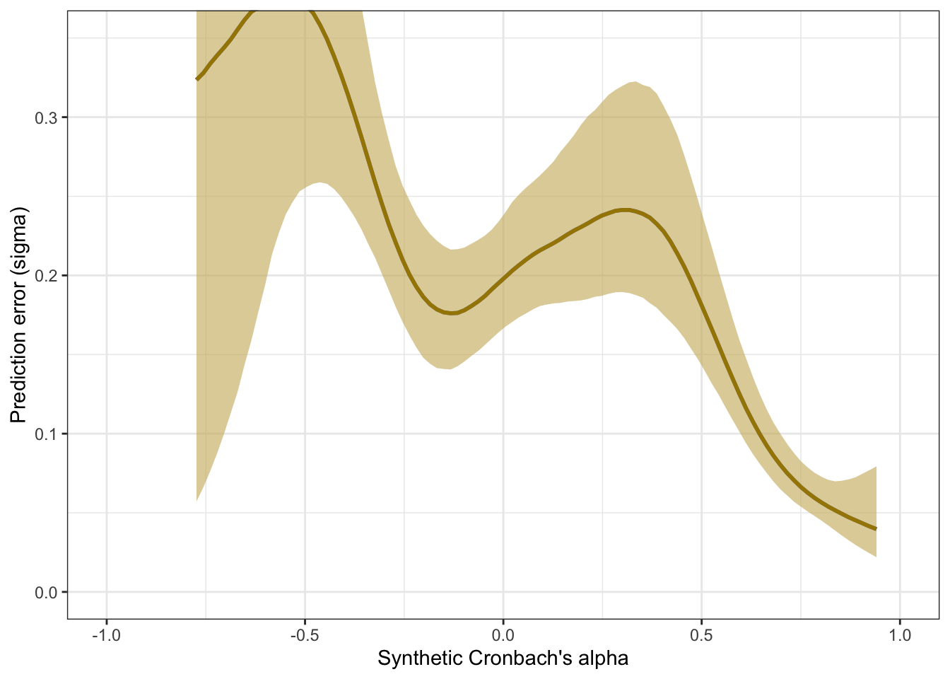

Scatter plot

ggplot(scales, aes(synthetic_alpha, empirical_alpha, 
                   color = str_detect(scale, "^random"), 
              ymin = empirical_alpha - empirical_alpha_se,
              ymax = empirical_alpha + empirical_alpha_se)) + 
  geom_abline(linetype = "dashed") +
  geom_point(alpha = 0.6, size = 1) +
  geom_smooth(aes(
    x = synthetic_alpha,
    y = estimate__,
    ymin = lower__,
    ymax = upper__,
  ), stat = "identity", 
  color = "#a48500",
  fill = "#EDC951",
  data = as.data.frame(pred$synthetic_alpha)) +
  scale_color_manual(values = c("#00A0B0", "#6A4A3C"),
                     guide = "none") +
  xlab("Synthetic Cronbach's alpha") + 
  ylab("Empirical Cronbach's alpha") +
  theme_bw() +
  coord_fixed(xlim = c(-1,1), ylim = c(-1,1)) -> plot_rels
plot_rels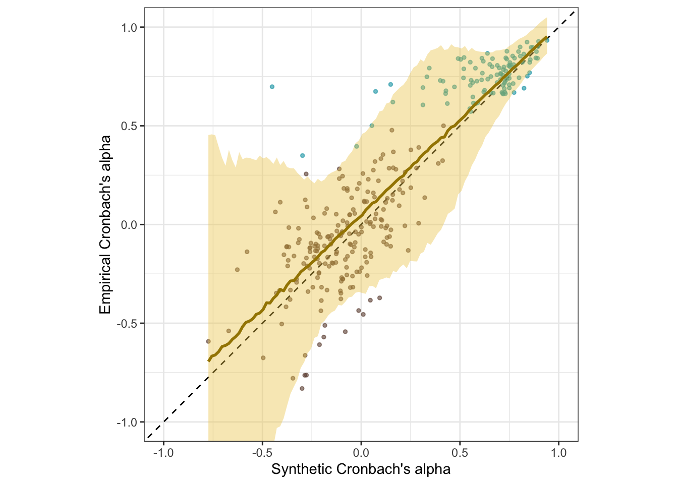

Interactive plot

(scales %>% 
  filter(type == "real") %>% 
  mutate(synthetic_alpha = round(synthetic_alpha, 2),
         empirical_alpha = round(empirical_alpha, 2),
         scale = str_replace_all(scale, "_+", " ")) %>% 
ggplot(., aes(synthetic_alpha, empirical_alpha, 
              # ymin = empirical_r - empirical_r_se, 
              # ymax = empirical_r + empirical_r_se, 
              label = scale)) + 
  geom_abline(linetype = "dashed") +
  geom_point(alpha = 0.3, size = 1, color = "#00A0B0") +
  xlab("Synthetic Cronbach's alpha") + 
  ylab("Empirical Cronbach's alpha") +
  theme_bw() +
  theme(legend.position='none') + 
  coord_fixed(xlim = c(NA,1), ylim = c(NA,1))) %>% 
  ggplotly()

Table

scales %>% 
  filter(type != "random") %>% 
  mutate(empirical_alpha = sprintf("%.2f±%.3f", empirical_alpha,
                               empirical_alpha_se),
         synthetic_alpha = sprintf("%.2f", synthetic_alpha),
         scale = str_replace_all(scale, "_+", " ")
         ) %>% 
  select(scale, empirical_alpha, synthetic_alpha, number_of_items) %>% 
  DT::datatable(rownames = FALSE,
                filter = "top")

scales %>% ungroup() %>% 
  summarise(mean(empirical_alpha), sd(empirical_alpha))

## # A tibble: 1 × 2
##   `mean(empirical_alpha)` `sd(empirical_alpha)`
##                     <dbl>                 <dbl>
## 1                   0.206                 0.449

scales %>% group_by(type) %>% 
  summarise(mean(empirical_alpha), sd(empirical_alpha),
            cor = broom::tidy(cor.test(synthetic_alpha, empirical_alpha)), n())

## # A tibble: 2 × 5
##   type   `mean(empirical_alpha)` `sd(empirical_alpha)` cor$estimate `n()`
##   <chr>                    <dbl>                 <dbl>        <dbl> <int>
## 1 random                 -0.0851                 0.246        0.587   200
## 2 real                    0.750                  0.101        0.628   107
## # ℹ 7 more variables: cor$statistic <dbl>, $p.value <dbl>, $parameter <int>,
## #   $conf.low <dbl>, $conf.high <dbl>, $method <chr>, $alternative <chr>

psychometric::cRRr(0.632, 0.0992, 0.235)

## # A tibble: 1 × 1
##   unrestricted
##          <dbl>
## 1        0.888

Robustness checks

Accuracy by whether scales were real or random

The SurveyBot3000 does not “know” whether scales were published in the literature or formed at random. Knowing what we do about the research literature in psychology, we can infer that published scales will usually exceed the Nunnally threshold of .70. Hence, we know that the synthetic alphas for published scales should rarely be below .70. If we regress synthetic alphas on empirical alphas separately for the scales taken from the literature, we see this as a bias (a positive regression intercept of .68 and a slope ≠ 1, .26). Still, the synthetic alpha estimates are predictive of empirical alphas with an accuracy of .65.

There is no clear bias for the random scales. When both are analyzed jointly, the clear selection bias for the published scales is mostly averaged out but is reflected in the slope exceeding 1.

scales %>% 
  group_by(type) %>% 
  summarise(broom::tidy(cor.test(synthetic_alpha, empirical_alpha)), sd_alpha = sd(empirical_alpha), n = n()) %>% 
  knitr::kable(digits = 2, caption = "Accuracy shown separately for randomly formed and real scales")

Accuracy shown separately for randomly formed and real scales

type	estimate	statistic	p.value	parameter	conf.low	conf.high	method	alternative	sd_alpha	n
random	0.59	10.20	0	198	0.49	0.67	Pearson’s product-moment correlation	two.sided	0.25	200
real	0.63	8.27	0	105	0.50	0.73	Pearson’s product-moment correlation	two.sided	0.10	107

scales %>% 
  group_by(type) %>% 
  summarise(broom::tidy(lm(empirical_alpha ~ synthetic_alpha)), n = n()) %>% 
  knitr::kable(digits = 2, caption = "Regression intercepts and slopes for randomly formed and real scales")

Regression intercepts and slopes for randomly formed and real scales

type	term	estimate	std.error	statistic	p.value	n
random	(Intercept)	-0.02	0.02	-1.33	0.19	200
random	synthetic_alpha	0.71	0.07	10.20	0.00	200
real	(Intercept)	0.58	0.02	26.09	0.00	107
real	synthetic_alpha	0.27	0.03	8.27	0.00	107

As in our Stage 1 submission

Here are the results if we calculate the accuracy and prediction error as in the Stage 1 submission. We now think this approach, by conditioning on random variation in the empirical correlations, gave a misleading picture of the accuracy and bias of the synthetic Cronbach’s alphas. Here we report the results if we conduct the analysis as in Stage 1 (but with the corrected SE of empirical alphas).

s1_scales <- scales %>%
  filter(number_of_items > 2) %>% 
  rowwise() %>%
  mutate(reverse_items = if_else(type == "random", list(reverse_items_by_1st), list(reverse_items)),
         r_real_rev = list(reverse_items(r_real, reverse_items)),
         pt_r_llm_rev = list(reverse_items(pt_r_llm, reverse_items)),
         r_llm_rev = list(reverse_items(r_llm, reverse_items))) %>%
  mutate(
    rel_real = list(psych::alpha(r_real_rev, keys = F, n.obs = N)$feldt),
    rel_llm = list(psych::alpha(r_llm_rev, keys = F, n.obs = N)$feldt),
    rel_pt_llm = list(psych::alpha(pt_r_llm_rev, keys = F, n.obs = N)$feldt)) %>%
  mutate(empirical_alpha = rel_real$alpha$raw_alpha,
         synthetic_alpha = rel_llm$alpha$raw_alpha,
         pt_synthetic_alpha = rel_pt_llm$alpha$raw_alpha) %>%
  mutate(
    empirical_alpha_se = mean(diff(unlist(psychometric::alpha.CI(empirical_alpha, k = number_of_items, N = N, level = 0.95))))/1.96) %>% 
      filter(empirical_alpha > 0)

s1_r <- broom::tidy(cor.test(s1_scales$empirical_alpha, s1_scales$synthetic_alpha))
s1_pt_r <- broom::tidy(cor.test(s1_scales$empirical_alpha, s1_scales$pt_synthetic_alpha))
                             
bind_rows(
  s1_pt_r %>% 
    mutate(model = "pre-trained", kind = "manifest") %>% 
    select(model, kind, accuracy = estimate, conf.low, conf.high),
  s1_r %>% 
    mutate(model = "fine-tuned", kind = "manifest") %>% 
    select(model, kind, accuracy = estimate, conf.low, conf.high),
  ) %>% 
  knitr::kable(digits = 2, caption = "Accuracy of synthetic alphas when empirical alphas are biased upward through adaptive item reversion and selection on positive alphas")

Accuracy of synthetic alphas when empirical alphas are biased upward through adaptive item reversion and selection on positive alphas

model	kind	accuracy	conf.low	conf.high
pre-trained	manifest	0.08	-0.03	0.19
fine-tuned	manifest	0.82	0.77	0.85

m_lmsynth_rel_scales_s1 <- brm(
  bf(empirical_alpha | mi(empirical_alpha_se) ~ synthetic_alpha,
     sigma ~ poly(synthetic_alpha, degree = 3)), data = s1_scales, 
  iter = 6000, control = list(adapt_delta = 0.9),
  file = "ignore/m_synth_rel_lm_as_stage_1")

pred <- conditional_effects(m_lmsynth_rel_scales_s1, method = "predict")
ggplot(s1_scales, aes(synthetic_alpha, empirical_alpha, 
                   color = str_detect(scale, "^random"), 
              ymin = empirical_alpha - empirical_alpha_se,
              ymax = empirical_alpha + empirical_alpha_se)) + 
  geom_abline(linetype = "dashed") +
  geom_point(alpha = 0.6, size = 1) +
  geom_smooth(aes(
    x = synthetic_alpha,
    y = estimate__,
    ymin = lower__,
    ymax = upper__,
  ), stat = "identity", 
  color = "#a48500",
  fill = "#EDC951",
  data = as.data.frame(pred$synthetic_alpha)) +  scale_color_manual(values = c("#00A0B0", "#6A4A3C"),
                     guide = "none") +
  xlab("Synthetic Cronbach's alpha") + 
  ylab("Empirical Cronbach's alpha") +
  theme_bw() +
  coord_fixed(xlim = c(-1, 1), ylim = c(-1,1))  -> s1_plot_rels
s1_plot_rels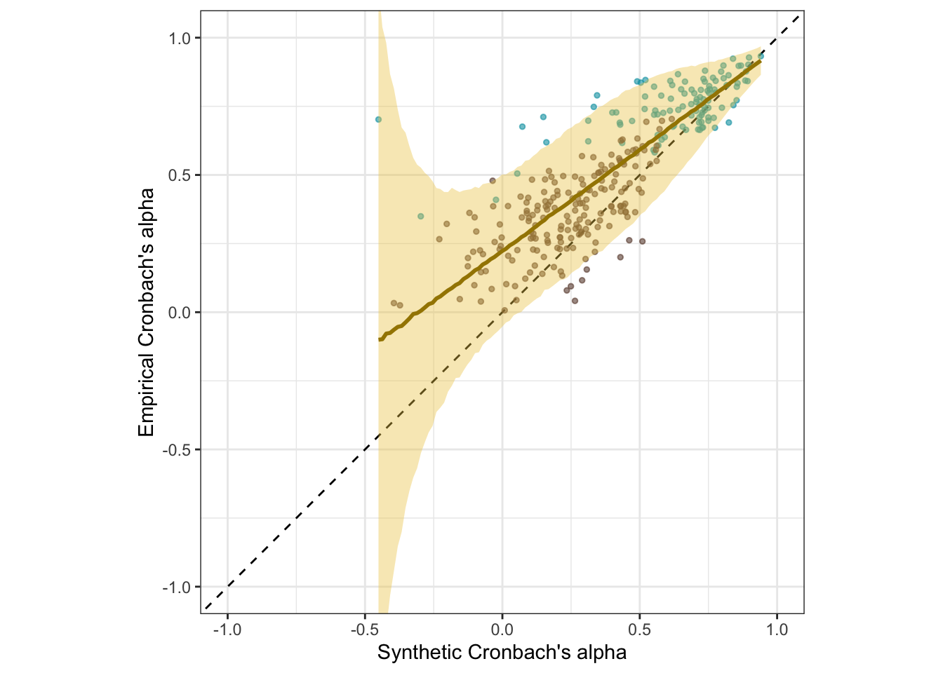

newdata <- m_lmsynth_rel_scales_s1$data %>% select(empirical_alpha, synthetic_alpha, empirical_alpha_se)
epreds <- epred_draws(newdata = newdata, obj = m_lmsynth_rel_scales_s1, re_formula = NA)
preds <- predicted_draws(newdata = newdata, obj = m_lmsynth_rel_scales_s1, re_formula = NA)
epred_preds <- epreds %>% left_join(preds)
by_draw <- epred_preds %>% group_by(.draw) %>% 
  summarise(
             mae = mean(abs(.epred - .prediction)),
            .epred = var(.epred),
            .prediction = var(.prediction),
            sigma = sqrt(.prediction - .epred),
            latent_r = sqrt(.epred/.prediction))

accuracy_bayes_rels_poly <- by_draw %>% mean_hdci(latent_r)

s1_plot_rels

bind_rows(
  r %>% 
    mutate(model = "fine-tuned", kind = "manifest") %>% 
    select(model, kind, accuracy = estimate, conf.low, conf.high),
  s1_r %>% 
    mutate(model = "fine-tuned, conditioned on empirical r", kind = "manifest") %>% 
    select(model, kind, accuracy = estimate, conf.low, conf.high),
  accuracy_bayes_rels %>% 
    mutate(model = "fine-tuned", kind = "latent outcome (Bayesian EIV)") %>% 
    select(model, kind, accuracy = latent_r, conf.low = .lower, conf.high = .upper),
  accuracy_bayes_rels_poly %>% 
    mutate(model = "fine-tuned, conditioned on empirical r", kind = "latent outcome (Bayesian EIV)") %>% 
    select(model, kind, accuracy = latent_r, conf.low = .lower, conf.high = .upper),
  ) %>% 
  knitr::kable(digits = 2, caption = "Accuracy of synthetic alphas when empirical alphas are biased upward through adaptive item reversion and selection on positive alphas")

Accuracy of synthetic alphas when empirical alphas are biased upward through adaptive item reversion and selection on positive alphas

model	kind	accuracy	conf.low	conf.high
fine-tuned	manifest	0.89	0.86	0.91
fine-tuned, conditioned on empirical r	manifest	0.82	0.77	0.85
fine-tuned	latent outcome (Bayesian EIV)	0.89	0.84	0.94
fine-tuned, conditioned on empirical r	latent outcome (Bayesian EIV)	0.85	0.77	0.92

Number of items as a trivial predictor

Although the number of items alone can of course predict Cronbach’s alpha, the synthetic alphas explain much more variance in empirical alphas.

scales %>% 
  ungroup() %>% 
  summarise(broom::tidy(cor.test(number_of_items, empirical_alpha)), sd_alpha = sd(empirical_alpha), n = n()) %>% 
  knitr::kable()

estimate	statistic	p.value	parameter	conf.low	conf.high	method	alternative	sd_alpha	n
0.136016	2.397701	0.0170994	305	0.0244477	0.2442379	Pearson’s product-moment correlation	two.sided	0.4490774	307

summary(lm(empirical_alpha ~ number_of_items, scales))

## 
## Call:
## lm(formula = empirical_alpha ~ number_of_items, data = scales)
## 
## Residuals:
##     Min      1Q  Median      3Q     Max 
## -1.0458 -0.3356 -0.1278  0.4982  0.7622 
## 
## Coefficients:
##                 Estimate Std. Error t value Pr(>|t|)  
## (Intercept)     0.098934   0.051336   1.927   0.0549 .
## number_of_items 0.016603   0.006925   2.398   0.0171 *
## ---
## Signif. codes:  0 '***' 0.001 '**' 0.01 '*' 0.05 '.' 0.1 ' ' 1
## 
## Residual standard error: 0.4456 on 305 degrees of freedom
## Multiple R-squared:  0.0185, Adjusted R-squared:  0.01528 
## F-statistic: 5.749 on 1 and 305 DF,  p-value: 0.0171

summary(lm(empirical_alpha ~ number_of_items + synthetic_alpha, scales))

## 
## Call:
## lm(formula = empirical_alpha ~ number_of_items + synthetic_alpha, 
##     data = scales)
## 
## Residuals:
##      Min       1Q   Median       3Q      Max 
## -0.58321 -0.09758  0.00643  0.10477  1.09299 
## 
## Coefficients:
##                  Estimate Std. Error t value Pr(>|t|)    
## (Intercept)      0.051451   0.024017   2.142    0.033 *  
## number_of_items -0.000593   0.003275  -0.181    0.856    
## synthetic_alpha  0.984484   0.029758  33.083   <2e-16 ***
## ---
## Signif. codes:  0 '***' 0.001 '**' 0.01 '*' 0.05 '.' 0.1 ' ' 1
## 
## Residual standard error: 0.2081 on 304 degrees of freedom
## Multiple R-squared:  0.7866, Adjusted R-squared:  0.7852 
## F-statistic: 560.4 on 2 and 304 DF,  p-value: < 2.2e-16

Is the accuracy lower for the pre-trained model?

ggplot(scales, aes(pt_synthetic_alpha, empirical_alpha, 
                   color = str_detect(scale, "^random"), 
              ymin = empirical_alpha - empirical_alpha_se,
              ymax = empirical_alpha + empirical_alpha_se)) + 
  geom_abline(linetype = "dashed") +
  geom_point(alpha = 0.6, size = 1) +
  scale_color_manual(values = c("#00A0B0", "#6A4A3C"),
                     guide = "none") +
  xlab("Synthetic Cronbach's alpha") + 
  ylab("Empirical Cronbach's alpha") +
  theme_bw() +
  coord_fixed(xlim = c(-1,1), ylim = c(-1,1)) -> pt_plot_rels
pt_plot_rels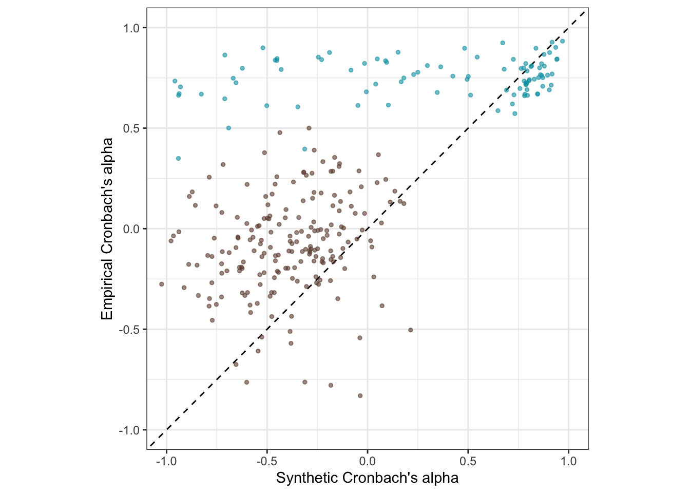

Synthetic Scale Correlations

manifest_scores = arrow::read_feather(file = file.path(data_path, glue("data/intermediate/{model_name}.raw.osf-bainbridge-2021-s2-0.scale_correlations.feather")))
pt_manifest_scores = arrow::read_feather(file = file.path(data_path, glue("data/intermediate/{pretrained_model_name}.raw.osf-bainbridge-2021-s2-0.scale_correlations.feather")))

n_distinct(manifest_scores$scale_a)

## [1] 112

manifest_scores <- manifest_scores %>%
 left_join(scales, by = c("scale_a" = "scale")) %>%
 left_join(scales, by = c("scale_b" = "scale"))

Accuracy

r <- broom::tidy(cor.test(manifest_scores$empirical_r, manifest_scores$synthetic_r))
pt_r <- broom::tidy(cor.test(pt_manifest_scores$empirical_r, pt_manifest_scores$synthetic_r))

se2 <- mean(manifest_scores$empirical_r_se^2)
model <- paste0('
    # Latent variables
    PearsonLatent =~ 1*empirical_r

    # Fixing error variances based on known standard errors
    empirical_r ~~ ',se2,'*empirical_r

    # Relationship between latent variables
    PearsonLatent ~~ synthetic_r
  ')

fit <- sem(model, data = manifest_scores)
pt_fit <- sem(model, data = pt_manifest_scores)


m_lmsynth_r_scales <- brm(
  bf(empirical_r | mi(empirical_r_se) ~ synthetic_r + (1|mm(scale_a, scale_b)),
     sigma ~ s(synthetic_r)), data = manifest_scores, 
  file = "ignore/m_synth_r_scales_lm8")

sd_synth <- sd(m_lmsynth_r_scales$data$synthetic_r)


newdata <- m_lmsynth_r_scales$data %>% select(empirical_r, synthetic_r, empirical_r_se)
epreds <- epred_draws(newdata = newdata, obj = m_lmsynth_r_scales, re_formula = NA)
preds <- predicted_draws(newdata = newdata, obj = m_lmsynth_r_scales, re_formula = NA)
epred_preds <- epreds %>% left_join(preds)
by_draw <- epred_preds %>% group_by(.draw) %>% 
  summarise(.epred = var(.epred),
            .prediction = var(.prediction),
            sigma = sqrt(.prediction - .epred),
            latent_r = sqrt(.epred/.prediction))

accuracy_bayes_scales <- by_draw %>% mean_hdci(latent_r)

bind_rows(
  pt_r %>% 
    mutate(model = "pre-trained", kind = "manifest") %>% 
    select(model, kind, accuracy = estimate, conf.low, conf.high),
  standardizedsolution(pt_fit) %>% 
    filter(lhs == "PearsonLatent", rhs ==  "synthetic_r") %>% 
    mutate(model = "pre-trained", kind = "latent outcome (SEM)") %>% 
    select(model, kind, accuracy = est.std, 
           conf.low = ci.lower, conf.high = ci.upper),
  r %>% 
    mutate(model = "fine-tuned", kind = "manifest") %>% 
    select(model, kind, accuracy = estimate, conf.low, conf.high),
  standardizedsolution(fit) %>% 
    filter(lhs == "PearsonLatent", rhs ==  "synthetic_r") %>% 
    mutate(model = "fine-tuned", kind = "latent outcome (SEM)") %>% 
    select(model, kind, accuracy = est.std, 
           conf.low = ci.lower, conf.high = ci.upper),
  accuracy_bayes_scales %>% 
    mutate(model = "fine-tuned", kind = "latent outcome (Bayesian EIV)") %>% 
    select(model, kind, accuracy = latent_r, conf.low = .lower, conf.high = .upper)
  ) %>% 
  knitr::kable(digits = 2)

model	kind	accuracy	conf.low	conf.high
pre-trained	manifest	0.33	0.30	0.35
pre-trained	latent outcome (SEM)	0.33	0.31	0.35
fine-tuned	manifest	0.87	0.86	0.87
fine-tuned	latent outcome (SEM)	0.88	0.87	0.89
fine-tuned	latent outcome (Bayesian EIV)	0.89	0.88	0.90

Prediction error plot according to synthetic estimate

m_lmsynth_r_scales

##  Family: gaussian 
##   Links: mu = identity; sigma = log 
## Formula: empirical_r | mi(empirical_r_se) ~ synthetic_r + (1 | mm(scale_a, scale_b)) 
##          sigma ~ s(synthetic_r)
##    Data: manifest_scores (Number of observations: 6245) 
##   Draws: 4 chains, each with iter = 2000; warmup = 1000; thin = 1;
##          total post-warmup draws = 4000
## 
## Smoothing Spline Hyperparameters:
##                           Estimate Est.Error l-95% CI u-95% CI Rhat Bulk_ESS
## sds(sigma_ssynthetic_r_1)     0.81      0.41     0.28     1.90 1.00     1061
##                           Tail_ESS
## sds(sigma_ssynthetic_r_1)     1472
## 
## Multilevel Hyperparameters:
## ~mmscale_ascale_b (Number of levels: 113) 
##               Estimate Est.Error l-95% CI u-95% CI Rhat Bulk_ESS Tail_ESS
## sd(Intercept)     0.07      0.01     0.06     0.08 1.01      743     1279
## 
## Regression Coefficients:
##                      Estimate Est.Error l-95% CI u-95% CI Rhat Bulk_ESS
## Intercept                0.01      0.01    -0.00     0.03 1.01      398
## sigma_Intercept         -2.15      0.01    -2.17    -2.13 1.00     3867
## synthetic_r              0.95      0.01     0.94     0.97 1.00     3232
## sigma_ssynthetic_r_1     0.02      1.20    -2.29     2.57 1.00     1202
##                      Tail_ESS
## Intercept                 770
## sigma_Intercept          2975
## synthetic_r              2772
## sigma_ssynthetic_r_1     1000
## 
## Draws were sampled using sample(hmc). For each parameter, Bulk_ESS
## and Tail_ESS are effective sample size measures, and Rhat is the potential
## scale reduction factor on split chains (at convergence, Rhat = 1).

kable(rmse_scales <- by_draw %>% mean_hdci(sigma), caption = "Average prediction error (RMSE)", digits = 2)

Average prediction error (RMSE)

sigma	.lower	.upper	.width	.point	.interval
0.12	0.11	0.12	0.95	mean	hdci

pred <- conditional_effects(m_lmsynth_r_scales, method = "predict")
plot_prediction_error_scales <- plot(conditional_effects(m_lmsynth_r_scales, dpar = "sigma"), plot = F)[[1]] + 
  theme_bw() + 
  geom_smooth(stat = "identity", color = "#a48500", fill = "#EDC951") + 
  xlab("Synthetic inter-scale correlation") + 
  ylab("Prediction error (sigma)")
plot_prediction_error_scales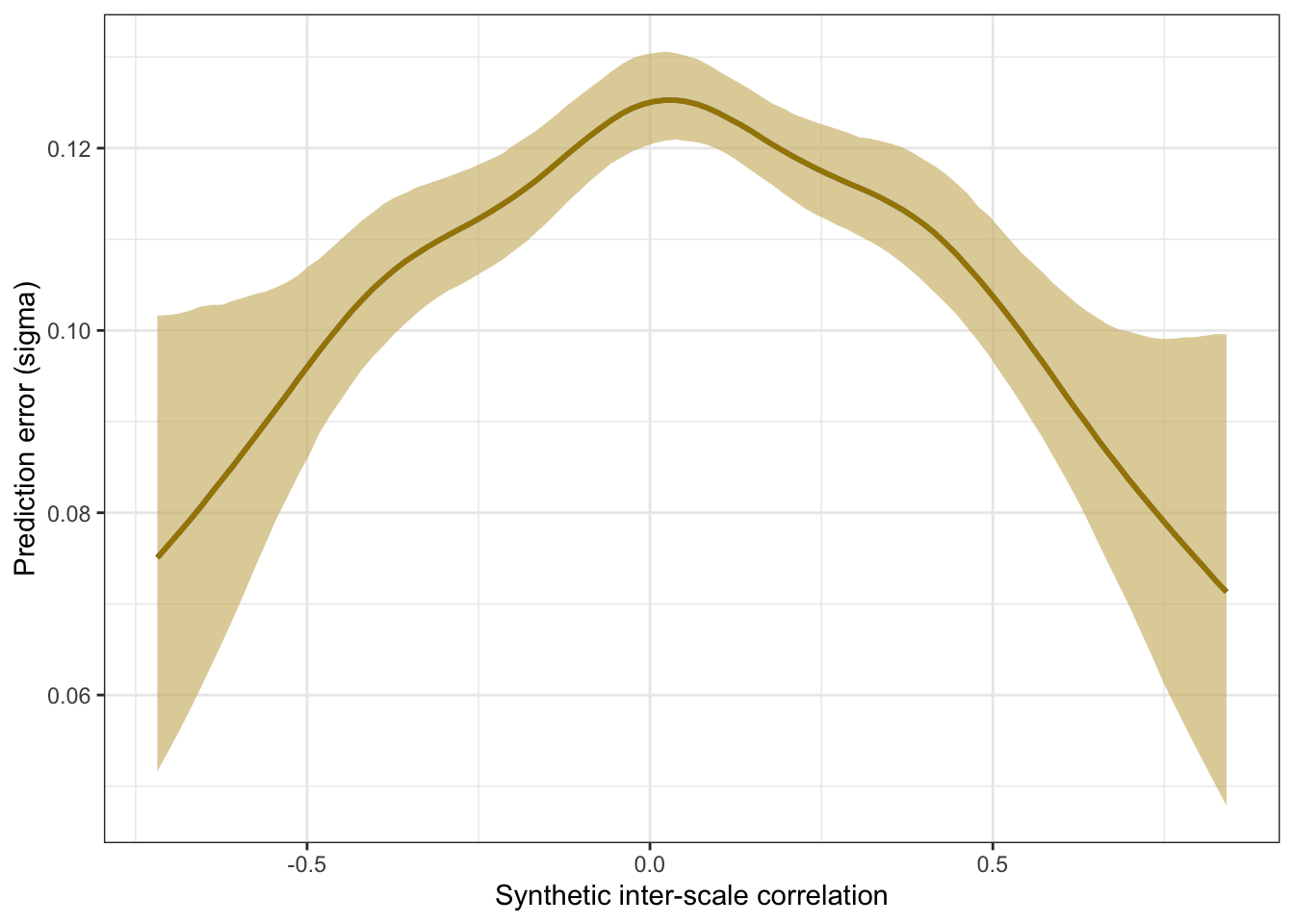

Scatter plot

ggplot(manifest_scores, aes(synthetic_r, empirical_r, 
              ymin = empirical_r - empirical_r_se,
              ymax = empirical_r + empirical_r_se)) + 
  geom_abline(linetype = "dashed") +
  geom_point(color = "#00A0B0", alpha = 0.3, size = 1) +
  geom_smooth(aes(
    x = synthetic_r,
    y = estimate__,
    ymin = lower__,
    ymax = upper__,
  ), stat = "identity", 
  color = "#a48500",
  fill = "#EDC951",
  data = as.data.frame(pred$synthetic_r)) +
  xlab("Synthetic inter-scale correlation") + 
  ylab("Empirical inter-scale correlation") +
  theme_bw() +
  coord_fixed(xlim = c(-1,1), ylim = c(-1,1)) -> plot_scales
plot_scales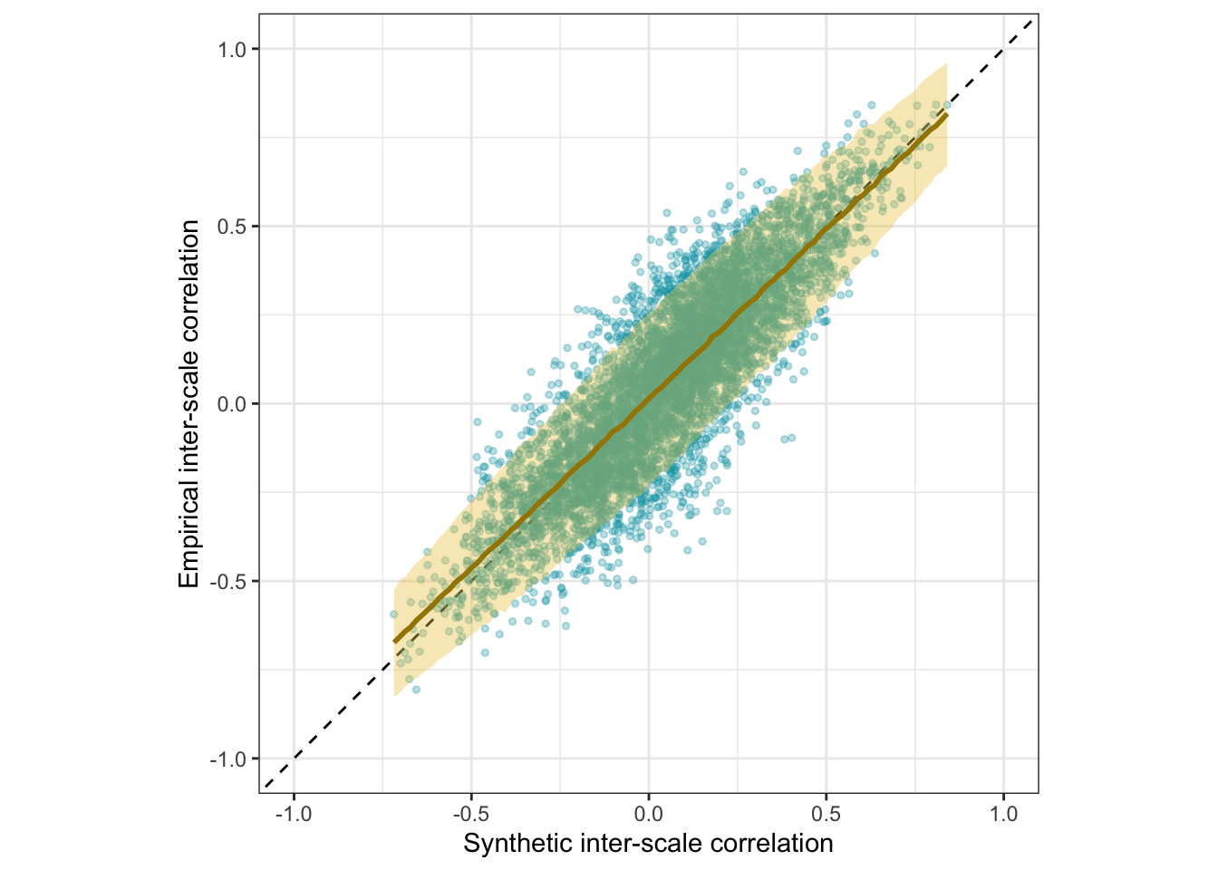

Interactive plot

(manifest_scores %>% 
  mutate(synthetic_r = round(synthetic_r, 2),
         empirical_r = round(empirical_r, 2),
         scales = str_replace_all(str_c(scale_a, "\n", scale_b),
                                  "_+", " ")) %>% 
ggplot(., aes(synthetic_r, empirical_r, 
              # ymin = empirical_r - empirical_r_se, 
              # ymax = empirical_r + empirical_r_se, 
              label = scales)) + 
  geom_abline(linetype = "dashed") +
  geom_point(color = "#00A0B0", alpha = 0.3, size = 1) +
  xlab("Synthetic inter-scale correlation") + 
  ylab("Empirical inter-scale correlation") +
  theme_bw() +
  coord_fixed(xlim = c(-1,1), ylim = c(-1,1))) %>% 
  ggplotly()

Table

manifest_scores %>% 
                mutate(empirical_r = sprintf("%.2f±%.3f", empirical_r,
                                             empirical_r_se),
                       synthetic_r = sprintf("%.2f", synthetic_r),
                       scale_a = str_replace_all(scale_a, "_+", " "),
                       scale_b = str_replace_all(scale_b, "_+", " ")
                       ) %>% 
                select(scale_a, scale_b, empirical_r, synthetic_r) %>% 
  DT::datatable(rownames = FALSE,
                filter = "top")

Robustness checks

Comparing spline and polynomial models for heteroscedasticity

m_lmsynth_r_scales_poly <- brm(
  bf(empirical_r | mi(empirical_r_se) ~ synthetic_r + (1|mm(scale_a, scale_b)),
     sigma ~ poly(synthetic_r, degree = 3)), data = manifest_scores, 
  file = "ignore/m_synth_r_scales_lm_poly")

newdata <- m_lmsynth_r_scales_poly$data %>% select(empirical_r, synthetic_r, empirical_r_se)
epreds <- epred_draws(newdata = newdata, obj = m_lmsynth_r_scales_poly, re_formula = NA)
preds <- predicted_draws(newdata = newdata, obj = m_lmsynth_r_scales_poly, re_formula = NA)
epred_preds <- epreds %>% left_join(preds)
by_draw <- epred_preds %>% group_by(.draw) %>% 
  summarise(.epred = var(.epred),
            .prediction = var(.prediction),
            sigma = sqrt(.prediction - .epred),
            latent_r = sqrt(.epred/.prediction))

accuracy_bayes_scales_poly <- by_draw %>% mean_hdci(latent_r)

bind_rows(
  accuracy_bayes_scales %>% 
    mutate(model = "spline", kind = "latent outcome (Bayesian EIV)") %>% 
    select(model, kind, accuracy = latent_r, conf.low = .lower, conf.high = .upper),
  accuracy_bayes_scales_poly %>% 
    mutate(model = "polynomial", kind = "latent outcome (Bayesian EIV)") %>% 
    select(model, kind, accuracy = latent_r, conf.low = .lower, conf.high = .upper)
) %>% 
  knitr::kable(digits = 2, caption = "Comparing spline and polynomial models for scale correlations")

Comparing spline and polynomial models for scale correlations

model	kind	accuracy	conf.low	conf.high
spline	latent outcome (Bayesian EIV)	0.89	0.88	0.9
polynomial	latent outcome (Bayesian EIV)	0.89	0.88	0.9

plot_prediction_error_scales_poly <- plot(conditional_effects(m_lmsynth_r_scales_poly, dpar = "sigma"), plot = F)[[1]] + 
  theme_bw() + 
  geom_smooth(stat = "identity", color = "#a48500", fill = "#EDC951") + 
  xlab("Synthetic inter-scale correlation") + 
  ylab("Prediction error (sigma)")
plot_prediction_error_scales_poly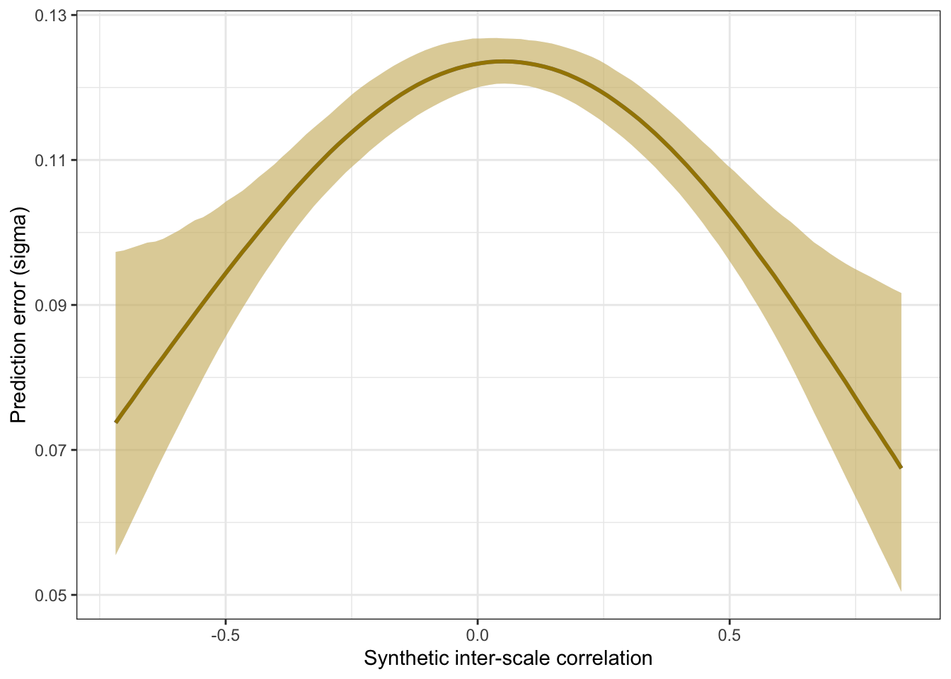

How does number of items across the two scales relate to accuracy?

by_item_number <- manifest_scores %>%
  mutate(items = number_of_items.x + number_of_items.y) %>%
  group_by(items) %>%
  summarise(broom::tidy(cor.test(empirical_r, synthetic_r)), pairwise_n = n()) 

by_item_number %>% 
  ggplot(aes(items, estimate, ymin = conf.low, ymax = conf.high)) + 
  geom_pointrange() +
  scale_y_continuous("Manifest accuracy (with 95% confidence interval)") +
  xlab("Number of items summed across scales")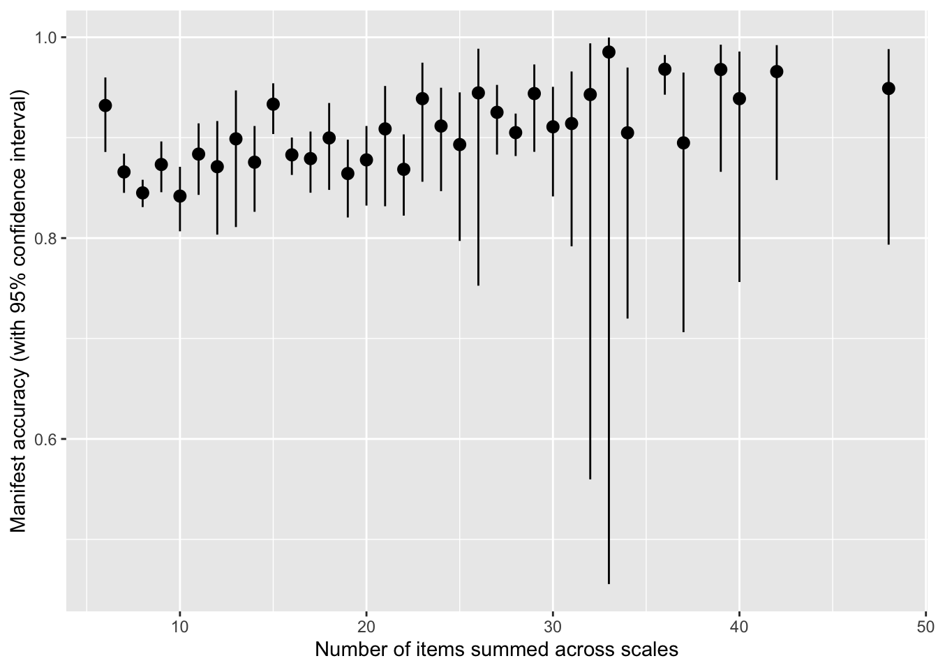

lm(estimate ~ items, by_item_number, weights = 1/(by_item_number$conf.high-by_item_number$conf.low))

## 
## Call:
## lm(formula = estimate ~ items, data = by_item_number, weights = 1/(by_item_number$conf.high - 
##     by_item_number$conf.low))
## 
## Coefficients:
## (Intercept)        items  
##    0.845728     0.002668

manifest_scores %>%
  filter(number_of_items.x >= 10, number_of_items.y >= 10) %>%
  summarise(cor = cor(empirical_r, synthetic_r), n())

## # A tibble: 1 × 2
##     cor `n()`
##   <dbl> <int>
## 1 0.926   300

Averages

scales %>% filter(type == "real") %>% ungroup() %>% 
  filter(number_of_items >= 3) %>% 
  summarise(median(number_of_items),
            mean(number_of_items))

## # A tibble: 1 × 2
##   `median(number_of_items)` `mean(number_of_items)`
##                       <int>                   <dbl>
## 1                         4                    6.79

Is the accuracy lower for the pre-trained model?

ggplot(pt_manifest_scores, aes(synthetic_r, empirical_r, 
              ymin = empirical_r - empirical_r_se,
              ymax = empirical_r + empirical_r_se)) + 
  geom_abline(linetype = "dashed") +
  geom_point(color = "#00A0B0", alpha = 0.3, size = 1) +
  xlab("Synthetic inter-scale correlation") + 
  ylab("Empirical inter-scale correlation") +
  theme_bw() +
  coord_fixed(xlim = c(-1,1), ylim = c(-1,1)) -> pt_plot_scales
pt_plot_scales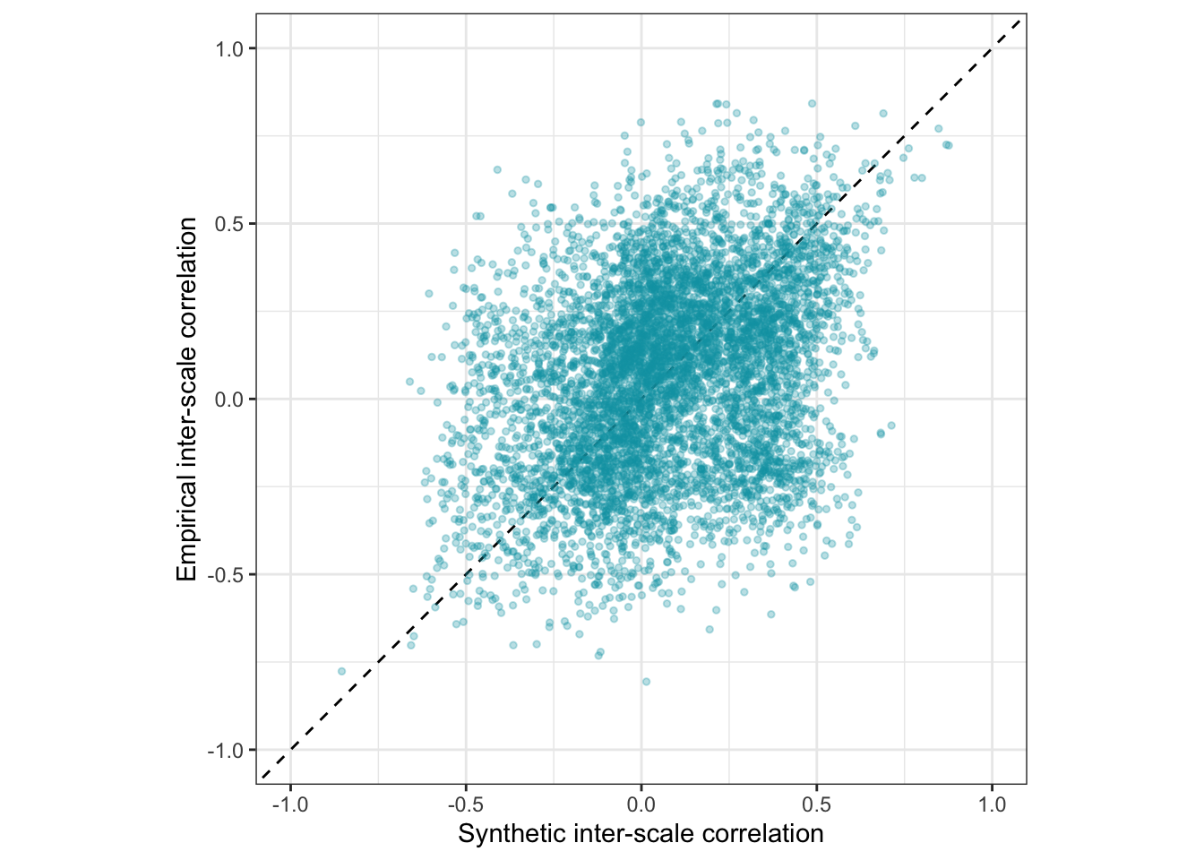

Combined plot

get_scale_point <- function(data, synthetic_approx, empirical_approx) {
  data %>%
    ungroup() %>% 
    # Find closest point to target coordinates
    mutate(dist = sqrt((synthetic_alpha - synthetic_approx)^2 + 
                      (empirical_alpha - empirical_approx)^2)) %>%
    arrange(dist) %>%
    slice(1) %>%
    select(synthetic_alpha, empirical_alpha)
}
get_scale_point_by_name <- function(data, name) {
  data %>%
    filter(scale == name) %>%
    slice(1) %>%
    select(synthetic_alpha, empirical_alpha, pt_synthetic_alpha)
}
ipip_e <- get_scale_point_by_name(scales, "International_Personality_Item_Pool_120_extraversion")
lot_o <- get_scale_point_by_name(scales, "Life_Orientation_Test_Optimism")
# get_scale_point_by_name <- function(data, var_1, var_2) {
#   data %>%
#     filter(variable_1 == scale_name) %>% 
#     select(synthetic_r, empirical_r)
# }

library(patchwork)
pt_plot_items2 <- pt_plot_items +
    annotate("text", size = 2.5, x = 0.5, y = -0.8, vjust = 1, hjust = 1, label = "r(I fear for the worst,\nI never worry about anything)", color = "#00A0B0") +
  annotate("segment", x = 0, y = -0.78, xend = 0.2761906, yend = -0.3459711, color = "#00A0B0", alpha = 0.7) +
  annotate("text", size = 2.5, x = -.1, y = 0.5, hjust = 1, label = "r(I get angry easily,\nI lose my temper)", color = "#00A0B0") + 
  annotate("segment", x = -.1, y = 0.5, xend = 0.6935711, yend = 0.7140546, color = "#00A0B0", alpha = 0.7)
  

plot_items2 <- plot_items +
  annotate("text", size = 3, x = -1, y = 0.98, vjust = 0, hjust = 0, label = with(accuracy_bayes_items, { sprintf("accuracy = %.2f [%.2f;%.2f]", latent_r, .lower, .upper) })) +
  annotate("text", size = 2.5, x = 0.5, y = -0.8, vjust = 1, hjust = 1, label = "r(I fear for the worst,\nI never worry about anything)", color = "#00A0B0") +
  annotate("segment", x = 0, y = -0.78, xend = -0.1104686, yend = -0.3459711, color = "#00A0B0", alpha = 0.7) +
  annotate("text", size = 2.5, x = -.1, y = 0.5, hjust = 1, label = "r(I get angry easily,\nI lose my temper)", color = "#00A0B0") + 
  annotate("segment", x = -.1, y = 0.5, xend = 0.8031979, yend = 0.7140546, color = "#00A0B0", alpha = 0.7)
  # annotate("text", size = 2.5, x = -0.5, y = -0.8, hjust = 0, label = "r(I love life,\nI avoid crowds)", color = "#00A0B0") +
  # annotate("segment", x = -.3, y = -0.7, xend = -0.23, yend = -0.28, color = "#00A0B0", alpha = 0.7) +
  # annotate("text", size = 2.5, x = -.3, y = 0.5, hjust = 1, label = "r(I work hard,\nI am diligent)", color = "#00A0B0") +
  # annotate("segment", x = -.3, y = .5, xend = .52, yend = .58, color = "#00A0B0", alpha = 0.7)


pt_plot_rels2 <- pt_plot_rels + 
  annotate("text", size = 2.5, x = 0.21, y = -0.2, hjust = 0, label = "IPIP Extraversion", color = "#00A0B0") +
  annotate("segment", x = 0.75, y = -0.2, xend = 0.87, yend = 0.90, color = "#00A0B0", alpha = 0.7) +
  annotate("text", size = 2.5, x = -0.02, y = 0.95, hjust = 0, label = "LOT Optimism", color = "#00A0B0") +
  annotate("segment", x = 0.11, y = 0.93, xend = -1.477226, yend = 0.71, color = "#00A0B0", alpha = 0.7)

p1 <- get_scale_point(scales, 0.30, 0.22)
p2 <- get_scale_point(scales, 0.12, -0.36) 
p3 <- get_scale_point(scales, -0.4, -0.90)


plot_rels2 <- plot_rels + 
  annotate("text", size = 3, x = -1, y = 0.98, vjust = 0, hjust = 0, 
           label = with(accuracy_bayes_rels, { sprintf("accuracy = %.2f [%.2f;%.2f]", latent_r, .lower, .upper) })) +
  annotate("text", size = 2.5, x = -0.2, y = -0.9, hjust = 0, label = "randomly formed scales", color = "#6A4A3C") +
  annotate("segment", x = 0.4, y = -0.85, xend = p1$synthetic_alpha, yend = p1$empirical_alpha, color = "#6A4A3C", alpha = 0.7) +
  annotate("segment", x = 0.4, y = -0.85, xend = p2$synthetic_alpha, yend = p2$empirical_alpha, color = "#6A4A3C", alpha = 0.7) +
  annotate("segment", x = 0.4, y = -0.85, xend = p3$synthetic_alpha, yend = p3$empirical_alpha, color = "#6A4A3C", alpha = 0.7) +

  annotate("text", size = 2.5, x = 0.21, y = -0.2, hjust = 0, label = "IPIP Extraversion", color = "#00A0B0") +
  annotate("segment", x = 0.75, y = -0.2, xend = 0.87, yend = 0.90, color = "#00A0B0", alpha = 0.7) +
  annotate("text", size = 2.5, x = -0.32, y = 0.86, hjust = 0, label = "LOT Optimism", color = "#00A0B0") +
  annotate("segment", x = 0, y = 0.83, xend = 0.49, yend = 0.71, color = "#00A0B0", alpha = 0.7)

pt_plot_scales2 <- pt_plot_scales +
  annotate("text", size = 2.5, x = -0.2, y = 0.8, hjust = 1, label = "r(BFI Neuroticism,\nIPIP Neuroticism)", color = "#00A0B0") +
  annotate("segment", x = -.2, y = 0.8, xend = 0.22, yend = .84, color = "#00A0B0", alpha = 0.7) +
  annotate("text", size = 2.5, x = -.1, y = -0.9, hjust = 0, label = "r(BFI Depression facet,\nLOT Optimism)", color = "#00A0B0") +
  annotate("segment", x = -.1, y = -.9, xend = -0.17, yend = -.63, color = "#00A0B0", alpha = 0.7)


plot_scales2 <- plot_scales +
  annotate("text", size = 3, x = -1, y = 0.98, vjust = 0, hjust = 0, label = with(accuracy_bayes_scales, { sprintf("accuracy = %.2f [%.2f;%.2f]", latent_r, .lower, .upper) })) +
  annotate("text", size = 2.5, x = -0.1, y = 0.5, hjust = 1, label = "r(BFI Neuroticism,\nIPIP Neuroticism)", color = "#00A0B0") +
  annotate("segment", x = -.1, y = 0.5, xend = .84, yend = .84, color = "#00A0B0", alpha = 0.7) +
  annotate("text", size = 2.5, x = -.15, y = -0.7, hjust = 0, label = "r(BFI Depression facet,\nLOT Optimism)", color = "#00A0B0") +
  annotate("segment", x = -.15, y = -.7, xend = -.34, yend = -.63, color = "#00A0B0", alpha = 0.7)


(pt_plot_items2  + ggtitle("Pre-trained model before domain adaptation and fine-tuning")+
    pt_plot_rels2 +
    pt_plot_scales2) /


(plot_items2 + ggtitle("SurveyBot 3000") +
    plot_rels2  +
    plot_scales2)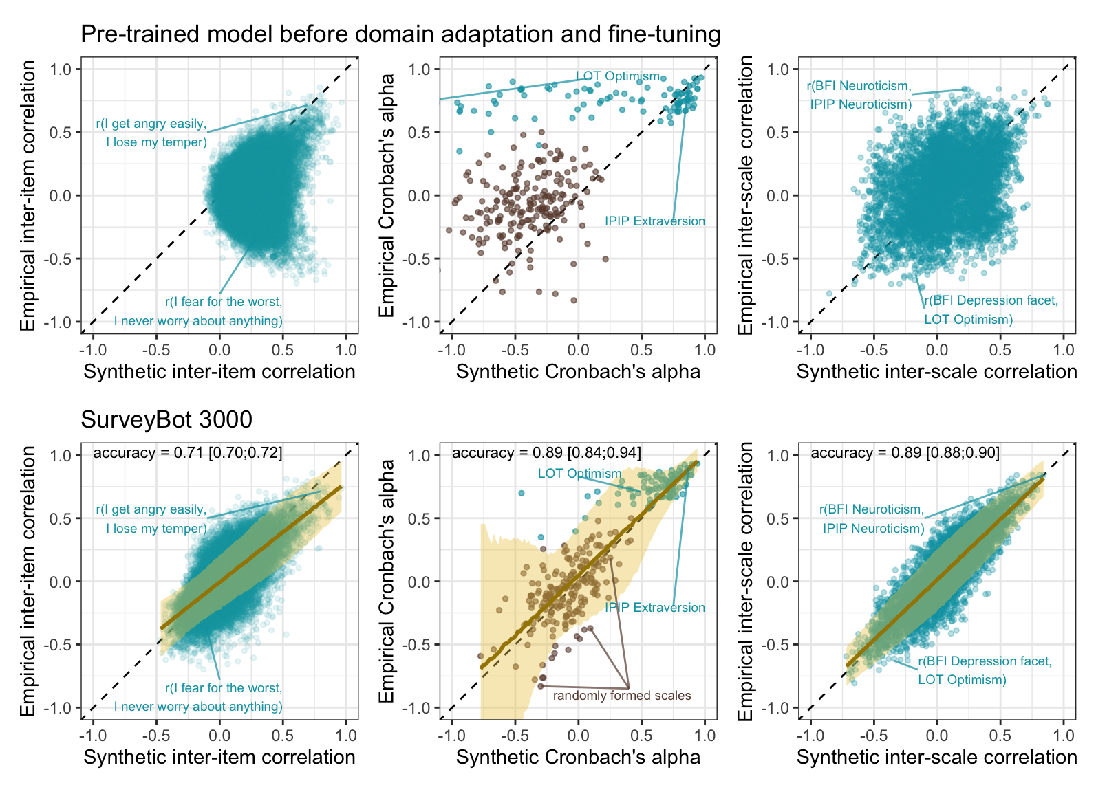

ggsave("Figure_pilot.pdf", width = 8.3, height = 6, device = grDevices::cairo_pdf)
ggsave("Figure_pilot.png", width = 8.3, height = 6)



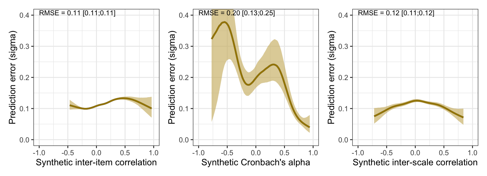
# ggsave("ignore/Figure_pilot.svg", width = 8.3, height = 5.5, device = svglite::svglite)

Prediction error plots

library(patchwork)

(plot_prediction_error_items + 
    coord_cartesian(xlim = c(-1, 1), ylim = c(0, 0.4)) +
    annotate("text", size = 3, x = -1, y = 0.4, vjust = 0, hjust = 0, label = with(rmse_items, { sprintf("RMSE = %.2f [%.2f;%.2f]", sigma, .lower, .upper) })) +
    
    plot_prediction_error_alpha + 
    coord_cartesian(xlim = c(-1, 1), ylim = c(0, 0.4))  +
    annotate("text", size = 3, x = -1, y = 0.4, vjust = 0, hjust = 0, label = with(rmse_alpha, { sprintf("RMSE = %.2f [%.2f;%.2f]", sigma, .lower, .upper) })) +
    
    plot_prediction_error_scales + 
    coord_cartesian(xlim = c(-1, 1), ylim = c(0, 0.4)) +
    annotate("text", size = 3, x = -1, y = 0.4, vjust = 0, hjust = 0, label = with(rmse_scales, { sprintf("RMSE = %.2f [%.2f;%.2f]", sigma, .lower, .upper) }))
)

ggsave("ignore/Figure_prediction_error_pilot.pdf", width = 8.3, height = 3, device = grDevices::cairo_pdf)
ggsave("ignore/Figure_prediction_error_pilot.png", width = 8.3, height = 3)