Language models accurately infer correlations between psychological items and = from text alone

Here, we apply the model to the data collected in our Registered Report validation sample on Nov 1, 2024.

knitr::opts_chunk$set(echo = TRUE, error = T, message = F, warning = F)
# Libraries and Settings

# Libs ---------------------------
library(knitr)
library(tidyverse)
library(arrow)
library(glue)
library(psych)
library(lavaan)
library(ggplot2)
library(plotly)
library(gridExtra)
library(broom)
library(broom.mixed)
library(brms)
library(tidybayes)
library(cmdstanr)
library(cowplot)

options(mc.cores = parallel::detectCores(), 
        brms.backend = "cmdstanr", 
        brms.file_refit = "never",
        width = 6000)

theme_set(theme_bw())

model_name = "ItemSimilarityTraining-20240502-trial12"
#model_name = "item-similarity-20231018-122504"
pretrained_model_name = "all-mpnet-base-v2"

data_path = glue("./data/intermediate/")
pretrained_data_path = glue("./data/intermediate/")

set.seed(42)
source("global_functions.R")


rr_validation <- arrow::read_feather(file = file.path(data_path, glue("{model_name}.raw.validation-study-2024-11-01.item_correlations.feather")))

pt_rr_validation <- arrow::read_feather(file = file.path(data_path, glue("{pretrained_model_name}.raw.validation-study-2024-11-01.item_correlations.feather")))

rr_validation_mapping_data = arrow::read_feather(
  file = file.path(data_path, glue("{model_name}.raw.validation-study-2024-11-01.mapping2.feather"))
) %>%
  rename(scale_0 = scale0,
         scale_1 = scale1)

rr_validation_human_data = arrow::read_feather(
  file = file.path(data_path, glue("{model_name}.raw.validation-study-2024-11-01.human.feather"))
)

rr_validation_scales <- arrow::read_feather(file.path(data_path, glue("{model_name}.raw.validation-study-2024-11-01.scales.feather"))
)

random_scales <- readRDS("data/intermediate/random_scales_rr.rds")

N <- rr_validation_human_data %>% summarise_all(~ sum(!is.na(.))) %>% min()
total_N <- nrow(rr_validation_human_data)

mapping_data <- rr_validation_mapping_data
items_by_scale <- bind_rows(
  rr_validation_scales %>% select(-keyed) %>% filter(scale_1 == "") %>% left_join(mapping_data %>% select(-scale_1), by = c("instrument", "scale_0")),
  rr_validation_scales %>% select(-keyed) %>% filter(scale_1 != "") %>% left_join(mapping_data, by = c("instrument", "scale_0", "scale_1"))
)

After exclusions, we had data on N=387 respondents. The item with the most missing values still had n=276.

Synthetic inter-item correlations

rr_validation_llm <- rr_validation %>%
  left_join(rr_validation_mapping_data %>% select(variable_1 = variable, InstrumentA = instrument, ScaleA = scale_0, SubscaleA = scale_1)) %>%
  left_join(rr_validation_mapping_data %>% select(variable_2 = variable, InstrumentB = instrument, ScaleB = scale_0, SubscaleB = scale_1)) %>% 
  left_join(pt_rr_validation %>% select(variable_1, variable_2, pt_synthetic_r = synthetic_r))

pt_rr_validation_llm <- pt_rr_validation %>%
  left_join(rr_validation_mapping_data %>% select(variable_1 = variable, InstrumentA = instrument, ScaleA = scale_0, SubscaleA = scale_1)) %>%
  left_join(rr_validation_mapping_data %>% select(variable_2 = variable, InstrumentB = instrument, ScaleB = scale_0, SubscaleB = scale_1))

Accuracy

se2 <- mean(rr_validation_llm$empirical_r_se^2)

r <- broom::tidy(cor.test(rr_validation_llm$empirical_r, rr_validation_llm$synthetic_r))
pt_r <- broom::tidy(cor.test(pt_rr_validation_llm$empirical_r, pt_rr_validation_llm$synthetic_r))

model <- paste0('
  # Latent variables
  PearsonLatent =~ 1*empirical_r

  # Fixing error variances based on known standard errors
  empirical_r ~~ ',se2,'*empirical_r

  # Relationship between latent variables
  PearsonLatent ~~ synthetic_r
')

fit <- sem(model, data = rr_validation_llm)
pt_fit <- sem(model, data = pt_rr_validation_llm)

pt_m_synth_r_items <- brm(
  bf(empirical_r | mi(empirical_r_se) ~ synthetic_r + (1|mm(variable_1, variable_2)),
     sigma ~ s(synthetic_r)), data = pt_rr_validation_llm, 
  file = "ignore/m_pt_synth_rr_r_items_lm")

newdata <- pt_m_synth_r_items$data %>% select(empirical_r, synthetic_r, empirical_r_se)
epreds <- epred_draws(newdata = newdata, obj = pt_m_synth_r_items, re_formula = NA, ndraws = 200)
preds <- predicted_draws(newdata = newdata, obj = pt_m_synth_r_items, re_formula = NA, ndraws = 200)
epred_preds <- epreds %>% left_join(preds)
by_draw <- epred_preds %>% group_by(.draw) %>% 
  summarise(.epred = var(.epred),
            .prediction = var(.prediction),
            sigma = sqrt(.prediction - .epred),
            latent_r = sqrt(.epred/.prediction))
rm(epred_preds)

pt_accuracy_bayes_items <- by_draw %>% mean_hdci(latent_r)


m_synth_r_items <- brm(
  bf(empirical_r | mi(empirical_r_se) ~ synthetic_r + (1|mm(variable_1, variable_2)),
     sigma ~ s(synthetic_r)), data = rr_validation_llm, 
  file = "ignore/m_synth_rr_r_items_lm")

sd_synth <- sd(m_synth_r_items$data$synthetic_r)

newdata <- m_synth_r_items$data %>% select(empirical_r, synthetic_r, empirical_r_se)
epreds <- epred_draws(newdata = newdata, obj = m_synth_r_items, re_formula = NA, ndraws = 200)
preds <- predicted_draws(newdata = newdata, obj = m_synth_r_items, re_formula = NA, ndraws = 200)
epred_preds <- epreds %>% left_join(preds)
by_draw <- epred_preds %>% group_by(.draw) %>% 
  summarise(
            mae = mean(abs(.epred - .prediction)),
            .epred = var(.epred),
            .prediction = var(.prediction),
            sigma = sqrt(.prediction - .epred),
            latent_r = sqrt(.epred/.prediction))
rm(epred_preds)

accuracy_bayes_items <- by_draw %>% mean_hdci(latent_r)


bind_rows(
  pt_r %>% 
    mutate(model = "pre-trained", kind = "manifest") %>% 
    select(model, kind, accuracy = estimate, conf.low, conf.high),
  standardizedsolution(pt_fit) %>% 
    filter(lhs == "PearsonLatent", rhs ==  "synthetic_r") %>% 
    mutate(model = "pre-trained", kind = "latent outcome (SEM)") %>% 
    select(model, kind, accuracy = est.std, 
           conf.low = ci.lower, conf.high = ci.upper),
  pt_accuracy_bayes_items %>% 
    mutate(model = "pre-trained", kind = "latent outcome (Bayesian EIV)") %>% 
    select(model, kind, accuracy = latent_r, conf.low = .lower, conf.high = .upper),
  r %>% 
    mutate(model = "fine-tuned", kind = "manifest") %>% 
    select(model, kind, accuracy = estimate, conf.low, conf.high),
  standardizedsolution(fit) %>% 
    filter(lhs == "PearsonLatent", rhs ==  "synthetic_r") %>% 
    mutate(model = "fine-tuned", kind = "latent outcome (SEM)") %>% 
    select(model, kind, accuracy = est.std, 
           conf.low = ci.lower, conf.high = ci.upper),
  accuracy_bayes_items %>% 
    mutate(model = "fine-tuned", kind = "latent outcome (Bayesian EIV)") %>% 
    select(model, kind, accuracy = latent_r, conf.low = .lower, conf.high = .upper)
  ) %>% 
  kable(digits = 2, caption = str_c("Accuracy for k=",nrow(rr_validation_llm)," item pairs (",n_distinct(c(rr_validation_llm$variable_1, rr_validation_llm$variable_1))," items) across language models and methods"))

Accuracy for k=30135 item pairs (245 items) across language models and methods

model	kind	accuracy	conf.low	conf.high
pre-trained	manifest	0.30	0.29	0.31
pre-trained	latent outcome (SEM)	0.31	0.30	0.32
pre-trained	latent outcome (Bayesian EIV)	0.33	0.32	0.35
fine-tuned	manifest	0.57	0.56	0.58
fine-tuned	latent outcome (SEM)	0.59	0.58	0.59
fine-tuned	latent outcome (Bayesian EIV)	0.59	0.58	0.61

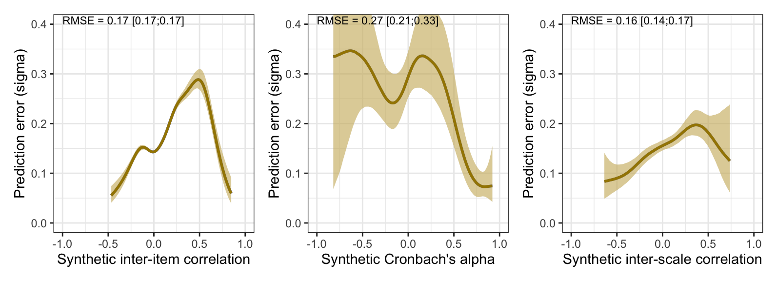
Prediction error plot according to synthetic estimate

m_synth_r_items

##  Family: gaussian
##   Links: mu = identity; sigma = log
## Formula: empirical_r | mi(empirical_r_se) ~ synthetic_r + (1 | mm(variable_1, variable_2))
##          sigma ~ s(synthetic_r)
##    Data: rr_validation_llm (Number of observations: 30135)
##   Draws: 4 chains, each with iter = 2000; warmup = 1000; thin = 1;
##          total post-warmup draws = 4000
##
## Smooth Terms:
##                           Estimate Est.Error l-95% CI u-95% CI Rhat Bulk_ESS Tail_ESS
## sds(sigma_ssynthetic_r_1)     2.37      0.68     1.39     4.08 1.00     1802     2183
##
## Group-Level Effects:
## ~mmvariable_1variable_2 (Number of levels: 246)
##               Estimate Est.Error l-95% CI u-95% CI Rhat Bulk_ESS Tail_ESS
## sd(Intercept)     0.08      0.00     0.08     0.09 1.00      991     1771
##
## Population-Level Effects:
##                      Estimate Est.Error l-95% CI u-95% CI Rhat Bulk_ESS Tail_ESS
## Intercept               -0.00      0.01    -0.01     0.01 1.00      562     1131
## sigma_Intercept         -1.81      0.00    -1.82    -1.80 1.00     6796     3280
## synthetic_r              0.98      0.01     0.96     0.99 1.00     7690     3289
## sigma_ssynthetic_r_1    -2.76      1.19    -5.00    -0.40 1.00     3883     3010
##
## Draws were sampled using sample(hmc). For each parameter, Bulk_ESS
## and Tail_ESS are effective sample size measures, and Rhat is the potential
## scale reduction factor on split chains (at convergence, Rhat = 1).

pred <- conditional_effects(m_synth_r_items, method = "predict")

kable(rmse_items <- by_draw %>% mean_hdci(sigma), caption = "Average prediction error (RMSE)", digits = 2)

Average prediction error (RMSE)

sigma	.lower	.upper	.width	.point	.interval
0.17	0.17	0.17	0.95	mean	hdci

kable(mae_items <- by_draw %>% mean_hdci(mae), caption = "Average prediction error (MAE)", digits = 2)

Average prediction error (MAE)

mae	.lower	.upper	.width	.point	.interval
0.13	0.13	0.13	0.95	mean	hdci

plot_prediction_error_items <- plot(conditional_effects(m_synth_r_items, dpar = "sigma"), plot = F)[[1]] + 
  theme_bw() + 
  xlab("Synthetic inter-item correlation") + 
  ylab("Prediction error (sigma)") +
  geom_smooth(stat = "identity", color = "#a48500", fill = "#EDC951")

plot_prediction_error_items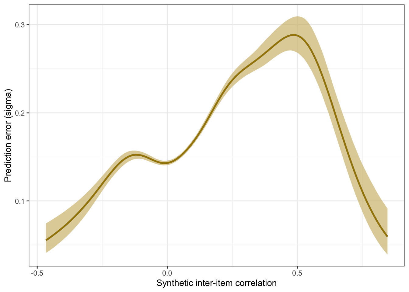

Scatter plot

ggplot(rr_validation_llm, aes(synthetic_r, empirical_r, 
              ymin = empirical_r - empirical_r_se,
              ymax = empirical_r + empirical_r_se)) + 
  geom_abline(linetype = "dashed") +
  geom_point(color = "#00A0B0", alpha = 0.03, size = 1) +
  geom_smooth(aes(
    x = synthetic_r,
    y = estimate__,
    ymin = lower__,
    ymax = upper__,
  ), stat = "identity", 
  color = "#a48500",
  fill = "#EDC951",
  data = as.data.frame(pred$synthetic_r)) +
  xlab("Synthetic inter-item correlation") + 
  ylab("Empirical inter-item correlation") +
  theme_bw() +
  coord_fixed(xlim = c(-1,1), ylim = c(-1,1)) -> plot_items
plot_items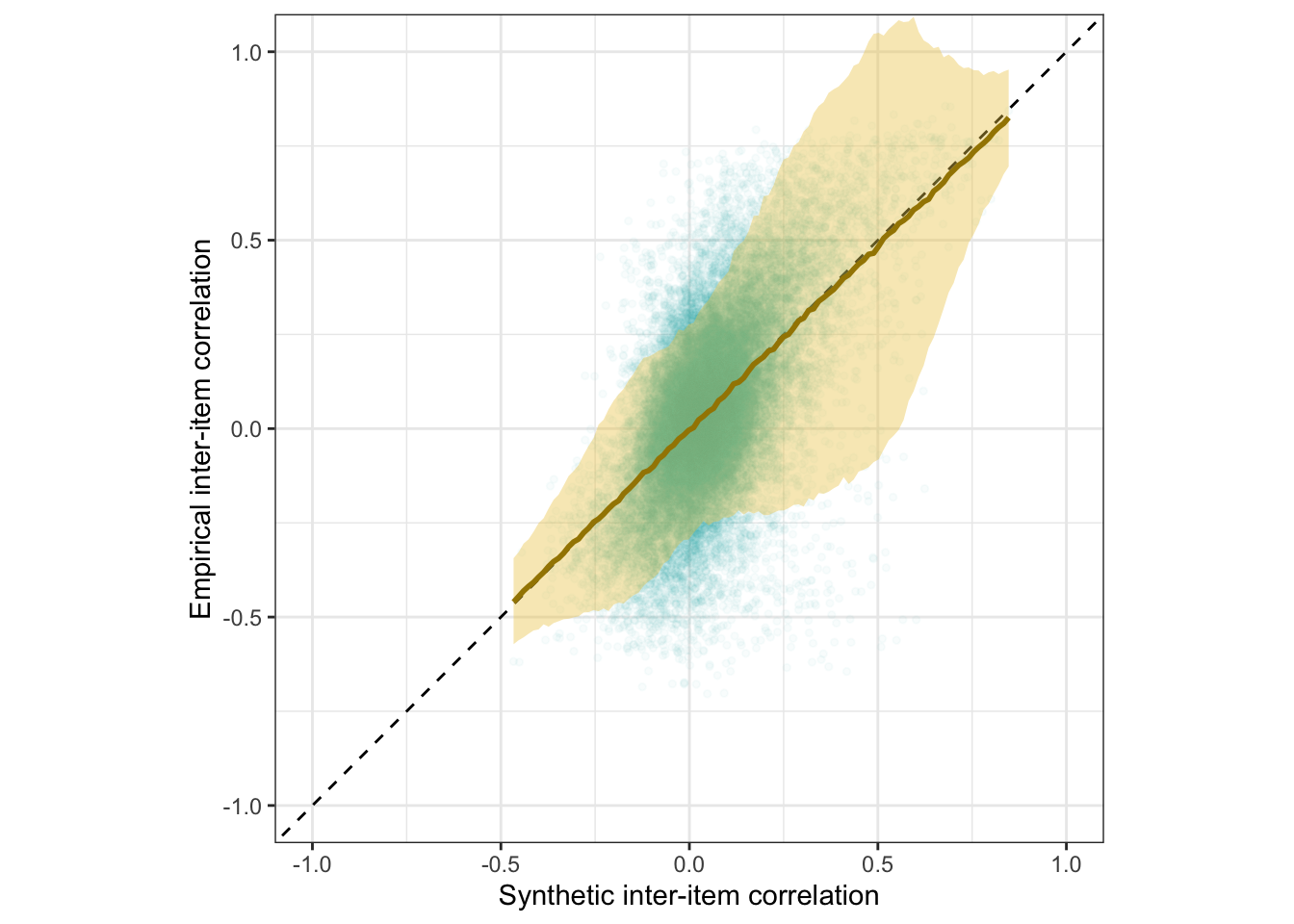

Interactive plot

This plot shows only 2000 randomly selected item pairs to conserve memory. A full interactive plot exists, but may react slowly.

item_pair_table <- rr_validation_llm %>% 
   left_join(rr_validation_mapping_data %>% select(variable_1 = variable,
                                             item_text_1 = item_text)) %>% 
   left_join(rr_validation_mapping_data %>% select(variable_2 = variable,
                                             item_text_2 = item_text))

# item_pair_table %>% filter(str_length(item_text_1) < 30, str_length(item_text_2) < 30) %>% 
#   left_join(pt_rr_validation_llm %>% rename(synthetic_r_pt = synthetic_r)) %>% 
#   select(item_text_1, item_text_2, empirical_r, synthetic_r, synthetic_r_pt) %>% View()
rio::export(item_pair_table, "ignore/item_pair_table_rr_unrounded.xlsx")
rio::export(item_pair_table, "ignore/item_pair_table_rr.feather")

(item_pair_table %>% 
  mutate(synthetic_r = round(synthetic_r, 2),
         empirical_r = round(empirical_r, 2),
         items = str_replace_all(str_c(item_text_1, "\n", item_text_2),
                                  "_+", " ")) %>% 
    sample_n(2000) %>%
ggplot(., aes(synthetic_r, empirical_r, 
              # ymin = empirical_r - empirical_r_se, 
              # ymax = empirical_r + empirical_r_se, 
              label = items)) + 
  geom_abline(linetype = "dashed") +
  geom_point(color = "#00A0B0", alpha = 0.3, size = 1) +
  xlab("Synthetic inter-item correlation") + 
  ylab("Empirical inter-item correlation") +
  theme_bw() +
  coord_fixed(xlim = c(-1,1), ylim = c(-1,1))) %>% 
  ggplotly()

item_pair_table_numeric <- item_pair_table

item_pair_table <- item_pair_table %>% 
  mutate(empirical_r = sprintf("%.2f±%.3f", empirical_r,
                                 empirical_r_se),
           synthetic_r = sprintf("%.2f", synthetic_r)) %>% 
  select(item_text_1, item_text_2, empirical_r, synthetic_r)
rio::export(item_pair_table, "item_pair_table_rr.xlsx")

Robustness checks

Comparing spline and polynomial models for heteroscedasticity

# For item correlations
m_synth_r_items_poly <- brm(
  bf(empirical_r | mi(empirical_r_se) ~ synthetic_r + (1|mm(variable_1, variable_2)),
     sigma ~ poly(synthetic_r, degree = 3)), data = rr_validation_llm, 
  file = "ignore/m_synth_rr_r_items_lm_poly")

newdata <- m_synth_r_items_poly$data %>% select(empirical_r, synthetic_r, empirical_r_se)
epreds <- epred_draws(newdata = newdata, obj = m_synth_r_items_poly, re_formula = NA, ndraws = 200)
preds <- predicted_draws(newdata = newdata, obj = m_synth_r_items_poly, re_formula = NA, ndraws = 200)
epred_preds <- epreds %>% left_join(preds)
by_draw <- epred_preds %>% group_by(.draw) %>% 
  summarise(.epred = var(.epred),
            .prediction = var(.prediction),
            sigma = sqrt(.prediction - .epred),
            latent_r = sqrt(.epred/.prediction))

accuracy_bayes_items_poly <- by_draw %>% mean_hdci(latent_r)

bind_rows(
  accuracy_bayes_items %>% 
    mutate(model = "spline", kind = "latent outcome (Bayesian EIV)") %>% 
    select(model, kind, accuracy = latent_r, conf.low = .lower, conf.high = .upper),
  accuracy_bayes_items_poly %>% 
    mutate(model = "polynomial", kind = "latent outcome (Bayesian EIV)") %>% 
    select(model, kind, accuracy = latent_r, conf.low = .lower, conf.high = .upper)
) %>% 
  knitr::kable(digits = 2, caption = "Comparing spline and polynomial models for item correlations")

Comparing spline and polynomial models for item correlations

model	kind	accuracy	conf.low	conf.high
spline	latent outcome (Bayesian EIV)	0.59	0.58	0.61
polynomial	latent outcome (Bayesian EIV)	0.59	0.58	0.60

plot_prediction_error_items_poly <- plot(conditional_effects(m_synth_r_items_poly, dpar = "sigma"), plot = F)[[1]] + 
  theme_bw() + 
  xlab("Synthetic inter-item correlation") + 
  ylab("Prediction error (sigma)") +
  geom_smooth(stat = "identity", color = "#a48500", fill = "#EDC951")

plot_prediction_error_items_poly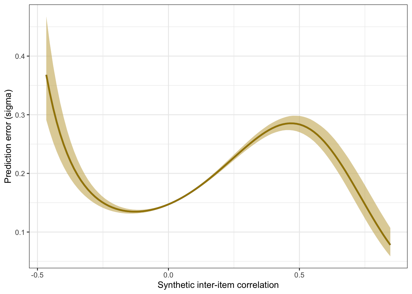

Accuracy by subject matter

Both items from same subject matter/domain

instruments <- rio::import("rr_used_measures.xlsx") %>% as_tibble()

rr_validation_llm_domain <- rr_validation_llm %>% 
  left_join(instruments %>% select(InstrumentA = Measure, DomainA = Domain), by = "InstrumentA") %>% 
  left_join(instruments %>% select(InstrumentB = Measure, DomainB = Domain), by = "InstrumentB") 

accuracy_within_domains <- rr_validation_llm_domain %>% 
  filter(DomainA == DomainB) %>% 
  group_by(DomainA) %>% 
  summarise(broom::tidy(cor.test(synthetic_r, empirical_r)), pt_cor = cor(pt_synthetic_r, empirical_r), rmse = sqrt(mean((empirical_r - synthetic_r)^2)), pt_rmse = sqrt(mean((empirical_r - pt_synthetic_r)^2)), sd_emp_r = sd(empirical_r), mean_abs_r = mean(abs(empirical_r)), mean_r = mean(empirical_r), pos_sign = mean(sign(empirical_r) > 0), n = n()) %>% 
  select(domain = DomainA, r = estimate, conf.low, conf.high, pt_cor, rmse, pt_rmse, n, sd_emp_r, mean_abs_r, mean_r, pos_sign) %>% 
  arrange(r)

accuracy_within_domains %>% 
  kable(digits = 2, caption = "Accuracy by domain when both items are from the same domain")

Accuracy by domain when both items are from the same domain

domain	r	conf.low	conf.high	pt_cor	rmse	pt_rmse	n	sd_emp_r	mean_abs_r	mean_r	pos_sign
attitudes	0.34	0.23	0.43	0.18	0.26	0.36	300	0.23	0.16	0.03	0.53
personality	0.42	0.37	0.47	0.06	0.20	0.33	1035	0.21	0.16	0.02	0.55
clinical	0.50	0.48	0.52	0.37	0.25	0.29	5050	0.28	0.26	0.16	0.78
social	0.72	0.69	0.74	0.25	0.19	0.31	1081	0.27	0.21	0.06	0.58
occupational	0.75	0.70	0.79	0.48	0.28	0.41	351	0.40	0.46	0.28	0.74

Items from one domain correlated with items in other domain

accuracy_between_domains <- bind_rows(rr_validation_llm_domain %>% 
  filter(DomainA != DomainB),
  rr_validation_llm_domain %>% 
  filter(DomainA != DomainB) %>% 
  rename(DomainA = DomainB, DomainB = DomainA)) %>% 
  group_by(DomainA) %>% 
  summarise(broom::tidy(cor.test(synthetic_r, empirical_r)), pt_cor = cor(pt_synthetic_r, empirical_r), rmse = sqrt(mean((empirical_r - synthetic_r)^2)), pt_rmse = sqrt(mean((empirical_r - pt_synthetic_r)^2)), sd_emp_r = sd(empirical_r), mean_abs_r = mean(abs(empirical_r)), mean_r = mean(empirical_r), pos_sign = mean(sign(empirical_r) > 0), n = n()) %>% 
  select(domain = DomainA, r = estimate, conf.low, conf.high, pt_cor, rmse, pt_rmse, n, sd_emp_r, mean_abs_r, mean_r, pos_sign) %>% 
  arrange(r)
accuracy_between_domains %>% 
  kable(digits = 2, caption = "Accuracy by domain when items are from different domains")

Accuracy by domain when items are from different domains

domain	r	conf.low	conf.high	pt_cor	rmse	pt_rmse	n	sd_emp_r	mean_abs_r	mean_r	pos_sign
attitudes	0.31	0.28	0.33	0.14	0.12	0.15	5525	0.11	0.09	0.02	0.58
personality	0.48	0.46	0.49	0.13	0.16	0.24	9200	0.17	0.14	0.03	0.56
clinical	0.54	0.53	0.56	0.18	0.17	0.25	14645	0.20	0.15	0.02	0.54
social	0.59	0.58	0.61	0.23	0.16	0.23	9353	0.20	0.16	0.04	0.59
occupational	0.65	0.64	0.66	0.23	0.16	0.28	5913	0.21	0.17	0.00	0.49

library(ggrepel)
dodge <- 0.6
bind_rows(
within = accuracy_within_domains,
across = accuracy_between_domains, .id = "kind") %>% 
  mutate(kind = fct_inorder(kind)) %>% 
ggplot(aes(x = domain, r, ymin = conf.low, ymax = conf.high, shape = kind, fill = kind)) +
  geom_col(aes( group = kind), position = position_dodge(width = dodge), width = 0.4) +
  geom_col(aes(y = pt_cor, group = kind), fill = "gray", position = position_dodge(width = dodge), , width = 0.4) +
  # geom_linerange(aes(ymin = pt_cor, ymax = r, group = kind), color = "gray", position = position_dodge(width = 1)) +
  # geom_point(aes(y = pt_cor, group = kind), color = "black", position = position_dodge(width = 1), size = 2.5) +
  geom_pointrange(position = position_dodge(width = dodge)) + 
  scale_fill_manual(values = c("#a48500", "#a48500"), guide = "none") + 
  scale_shape_manual(values = c("within" = 19, "across" = 4), guide = "none") +
  # scale_color_viridis_d(end = 0.7, option = "A", guide = "none") +
  scale_y_continuous("Manifest accuracy of synthetic item pair correlations", limits = c(0, 1), expand = c(0, 0)) +
  xlab("Item domain") +
  annotate("text", label = "SBERT", x = 2.85, y = 0.24,  angle = 90) +
  annotate("text", label = "SurveyBot3000", x = 3.15, y = 0.43,  angle = 90) +
  annotate("text_repel", label = "within domain", x = 2.85, y = .745, force = 2, hjust = 1.15, vjust = -2) +
  annotate("text_repel", label = "across domains", x = 3.15, y = .65, force = 2, hjust = -.15, vjust = -2) +
  geom_text(aes(label = sprintf("%.2f", r), hjust = if_else(kind == "within", 1.3, -0.3)), vjust = -0.4, size = 3, position = position_dodge(width = dodge))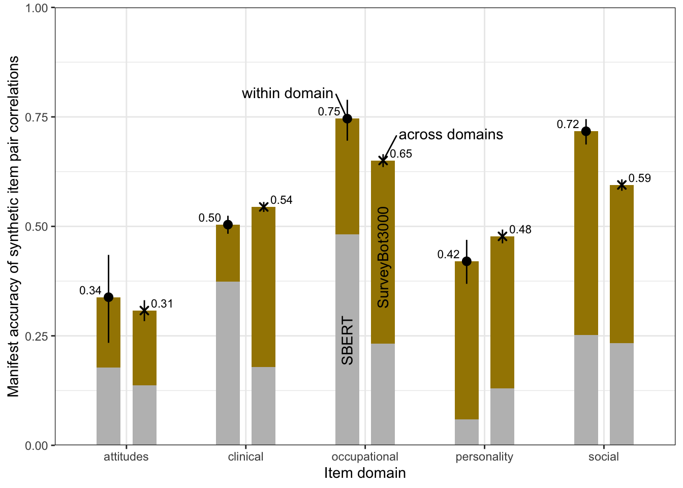

ggsave("Figure_rr_domain.png", width = 6, height = 5)

Accuracy by instrument

accuracy_between_instruments <- bind_rows(rr_validation_llm_domain %>% 
  filter(InstrumentA != InstrumentB),
  rr_validation_llm_domain %>% 
  filter(InstrumentA != InstrumentB) %>% 
  rename(InstrumentA = InstrumentB, InstrumentB = InstrumentA)) %>% 
  group_by(InstrumentA) %>% 
  summarise(broom::tidy(cor.test(synthetic_r, empirical_r)), pt_cor = cor(pt_synthetic_r, empirical_r), sd_emp_r = sd(empirical_r), n = n()) %>% 
  select(instrument = InstrumentA, r = estimate, conf.low, conf.high, pt_cor, n, sd_emp_r) %>% 
  arrange(r) %>% 
  mutate(instrument = fct_inorder(instrument))

accuracy_between_instruments %>% 
  kable(digits = 2, caption = "Accuracy by instrument (for items belonging to other instruments)")

Accuracy by instrument (for items belonging to other instruments)

instrument	r	conf.low	conf.high	pt_cor	n	sd_emp_r
Authoritarianism Short Scale	0.20	0.16	0.24	0.23	2133	0.11
New Ecological Paradigm Scale	0.20	0.16	0.24	0.12	2360	0.12
Disgust Avoidance Questionnaire	0.24	0.21	0.27	0.18	3893	0.08
Perth Alexithymia Questionnaire	0.34	0.30	0.37	0.15	2360	0.17
Moral Foundations Questionnaire	0.34	0.31	0.37	0.26	2585	0.12
Attitudes Toward AI in Defense Scale	0.35	0.30	0.39	0.11	1440	0.10
HEXACO-60	0.36	0.34	0.38	0.08	6480	0.15
Fear of COVID-19 Scale	0.36	0.32	0.40	0.23	1673	0.10
Survey Attitude Scale	0.37	0.33	0.40	0.12	2133	0.10
Perceived Stress Scale	0.50	0.48	0.53	0.18	3248	0.27
Perseverative Thinking Questionnaire	0.51	0.49	0.54	0.31	3465	0.28
Obsessive–Compulsive Inventory (Revised)	0.56	0.54	0.58	0.23	4104	0.17
Chronotype Questionnaire	0.60	0.58	0.62	0.19	3680	0.21
Revised Adult Attachment Scale	0.62	0.59	0.64	0.23	2585	0.21
Work Gratitude Scale	0.67	0.65	0.69	0.36	2360	0.19
Center for Epidemiological Studies Depression Scale	0.68	0.67	0.70	0.38	4520	0.28
Utrecht Work Engagement Scale (Short Version)	0.70	0.67	0.72	0.36	2133	0.24
Oldenburg Burnout Inventory (English Translation)	0.71	0.68	0.73	0.30	1904	0.26
UCLA Loneliness Scale (Short Form)	0.72	0.69	0.74	0.33	1904	0.27
Positive and Negative Affect Schedule	0.72	0.70	0.74	0.28	1904	0.28

accuracy_within_instruments <- rr_validation_llm %>% 
  filter(InstrumentA == InstrumentB) %>% 
  left_join(items_by_scale %>% select(variable_1 = variable, keyed = keyed) %>% distinct()) %>% 
  group_by(InstrumentA) %>% 
  summarise(broom::tidy(cor.test(synthetic_r, empirical_r)), pt_cor = cor(pt_synthetic_r, empirical_r), sd_emp_r = sd(empirical_r), n = n(), reverse_item_percentage = sum(keyed == -1, na.rm = TRUE)/n()) %>% 
  select(instrument = InstrumentA, r = estimate, conf.low, conf.high, pt_cor, n, sd_emp_r, reverse_item_percentage) %>% 
  arrange(r) %>% 
  mutate(instrument = factor(instrument, levels = levels(accuracy_between_instruments$instrument)))
  
accuracy_within_instruments %>% 
  mutate(accuracy = sprintf("%.2f [%.2f;%.2f]", r, conf.low, conf.high)) %>% 
  select(-c(r, conf.low, conf.high)) %>% 
  relocate(accuracy, .before = pt_cor) %>%
  rename(pt_accuracy = pt_cor) %>% 
  kable(digits = 2, caption = "Accuracy by instrument (within items belonging to the same instrument)")

Accuracy by instrument (within items belonging to the same instrument)

instrument	accuracy	pt_accuracy	n	sd_emp_r	reverse_item_percentage
New Ecological Paradigm Scale	0.02 [-0.28;0.31]	-0.08	45	0.39	0.47
Moral Foundations Questionnaire	0.03 [-0.23;0.30]	0.08	55	0.20	0.00
HEXACO-60	0.35 [0.27;0.43]	0.04	435	0.20	0.50
Fear of COVID-19 Scale	0.39 [-0.05;0.70]	0.34	21	0.07	0.00
Perseverative Thinking Questionnaire	0.45 [0.28;0.59]	0.15	105	0.09	0.00
Authoritarianism Short Scale	0.47 [0.17;0.69]	0.39	36	0.10	0.00
Perceived Stress Scale	0.50 [0.33;0.64]	0.31	91	0.50	0.48
Chronotype Questionnaire	0.57 [0.44;0.68]	0.22	120	0.38	0.62
Survey Attitude Scale	0.58 [0.31;0.76]	0.39	36	0.39	0.08
Disgust Avoidance Questionnaire	0.62 [0.50;0.71]	0.56	136	0.06	0.00
Work Gratitude Scale	0.64 [0.43;0.79]	0.41	45	0.10	0.00
Revised Adult Attachment Scale	0.71 [0.55;0.82]	0.23	55	0.49	0.44
Obsessive–Compulsive Inventory (Revised)	0.71 [0.62;0.78]	0.57	153	0.11	0.00
Utrecht Work Engagement Scale (Short Version)	0.79 [0.62;0.89]	0.62	36	0.12	0.00
Perth Alexithymia Questionnaire	0.80 [0.67;0.89]	0.70	45	0.14	0.00
Oldenburg Burnout Inventory (English Translation)	0.84 [0.68;0.92]	0.38	28	0.54	0.57
Attitudes Toward AI in Defense Scale	0.86 [0.63;0.95]	0.41	15	0.39	0.00
Center for Epidemiological Studies Depression Scale	0.87 [0.84;0.90]	0.55	190	0.50	0.21
UCLA Loneliness Scale (Short Form)	0.93 [0.85;0.97]	0.20	28	0.55	0.25
Positive and Negative Affect Schedule	0.94 [0.87;0.97]	0.50	28	0.51	0.00

bind_rows(
within = accuracy_within_instruments,
across = accuracy_between_instruments, .id = "kind") %>% 
ggplot(aes(x = instrument, r, ymin = conf.low, ymax = conf.high, shape = kind)) +
  geom_point(aes(y = pt_cor, group = kind), color = "gray", position = position_dodge(width = 0.3)) +
  geom_linerange(aes(ymin = pt_cor, ymax = r, group = kind), color = "gray", position = position_dodge(width = 0.3)) +
  geom_pointrange(position = position_dodge(width = 0.3)) + 
  scale_shape_manual(values = c("within" = 19, "across" = 4), guide = "none") +
  scale_color_viridis_d(end = 0.7, option = "A", guide = F) +
  scale_y_continuous("Manifest accuracy") +
  geom_text(aes(label = sprintf("%.2f", r)), vjust = -1, position = position_dodge(width = 0.3)) +
  coord_flip()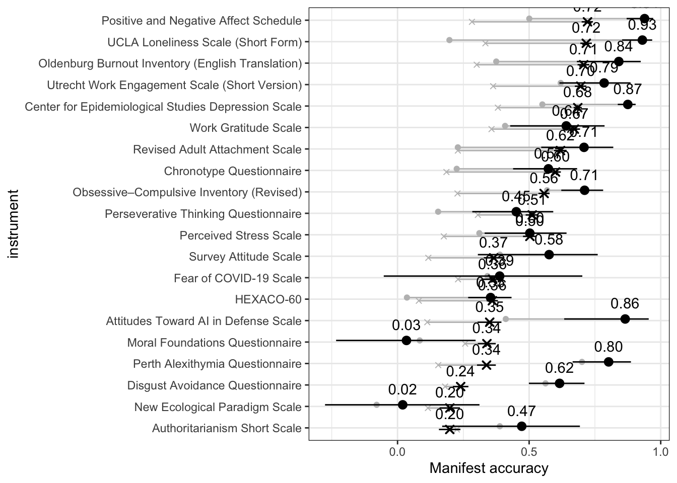

Accuracy by item properties

r_by_item <- rr_validation_llm %>% 
  # filter(InstrumentA == InstrumentB, SubscaleA == SubscaleB, ScaleA == ScaleB) %>% 
  left_join(items_by_scale %>% select(variable_1 = variable, keyed = keyed, item_text) %>% distinct()) %>% 
  group_by(variable_1) %>% 
  filter(n() > 3) %>% 
  summarise(broom::tidy(cor.test(synthetic_r, empirical_r)), pt_cor = cor(pt_synthetic_r, empirical_r), sd_emp_r = sd(empirical_r), n = n(), reverse_item_percentage = sum(keyed == -1)/n(), item_text_length = first(str_length(item_text))) %>% 
  select(r = estimate, conf.low, conf.high, pt_cor, n, sd_emp_r, reverse_item_percentage, item_text_length) %>% 
  arrange(r)

r_by_item %>% ggplot(aes(item_text_length, r, color = factor(reverse_item_percentage))) + 
  scale_color_viridis_d("reversed", end = 0.8) +
  geom_point() + geom_smooth(method = "lm") +
  ylab("Accuracy (r)")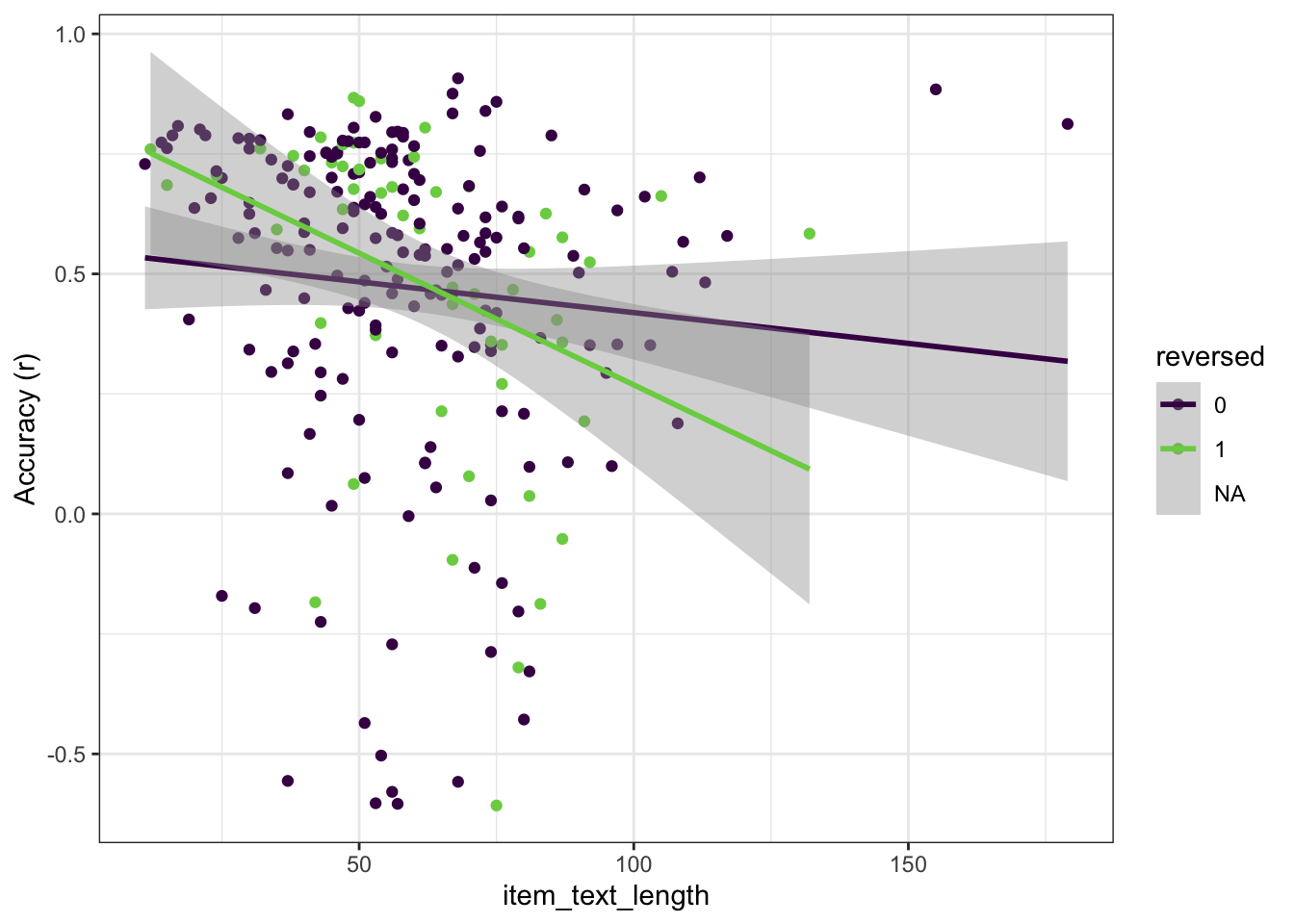

Does the item contain a first person singular pronoun

item_pair_table_numeric <- item_pair_table_numeric %>% 
  mutate(pronoun_1 = str_detect(item_text_1, "\\b(I|me|my|mine|myself|Me|My|Mine|Myself)\\b"),
         pronoun_2 = str_detect(item_text_2, "\\b(I|me|my|mine|myself|Me|My|Mine|Myself)\\b")) %>% 
  mutate(pronouns_in_item_pair = case_when(
    pronoun_1 == F & pronoun_2 == F ~ "neither",
    pronoun_1 == T & pronoun_2 == T ~ "both",
    TRUE ~ "one"
  )) %>% 
  mutate(item_text_length_1 = str_length(item_text_1),
         item_text_length_2 = str_length(item_text_2),
         item_text_length = (item_text_length_1+item_text_length_2)/2) %>% 
  left_join(items_by_scale %>% select(variable_1 = variable, keyed_1 = keyed) %>% distinct()) %>% 
  left_join(items_by_scale %>% select(variable_2 = variable, keyed_2 = keyed) %>% distinct()) %>% 
  mutate(reversed_items = case_when(
    keyed_1 == 1 & keyed_2 == 1 ~ "neither",
    keyed_1 == -1 & keyed_2 == -1 ~ "both",
    TRUE ~ "one"
  ))


options(scipen = 10)
summary(lm(empirical_r ~ synthetic_r * (pronouns_in_item_pair + reversed_items + item_text_length), item_pair_table_numeric))

##
## Call:
## lm(formula = empirical_r ~ synthetic_r * (pronouns_in_item_pair +
##     reversed_items + item_text_length), data = item_pair_table_numeric)
##
## Residuals:
##      Min       1Q   Median       3Q      Max
## -1.02473 -0.10214  0.00171  0.10758  0.76774
##
## Coefficients:
##                                             Estimate  Std. Error t value   Pr(>|t|)
## (Intercept)                              -0.01571570  0.00656285  -2.395    0.01664 *
## synthetic_r                               1.54349104  0.04100884  37.638    < 2e-16 ***
## pronouns_in_item_pairneither              0.00623656  0.00566222   1.101    0.27072
## pronouns_in_item_pairone                 -0.00669539  0.00242107  -2.765    0.00569 **
## reversed_itemsneither                     0.02400836  0.00529971   4.530 0.00000592 ***
## reversed_itemsone                        -0.01776464  0.00542131  -3.277    0.00105 **
## item_text_length                          0.00017506  0.00006971   2.511    0.01204 *
## synthetic_r:pronouns_in_item_pairneither -0.63680974  0.03385991 -18.807    < 2e-16 ***
## synthetic_r:pronouns_in_item_pairone     -0.28711562  0.02033846 -14.117    < 2e-16 ***
## synthetic_r:reversed_itemsneither        -0.15446421  0.03441803  -4.488 0.00000722 ***
## synthetic_r:reversed_itemsone            -0.33280281  0.03602897  -9.237    < 2e-16 ***
## synthetic_r:item_text_length             -0.00473406  0.00045087 -10.500    < 2e-16 ***
## ---
## Signif. codes:  0 '***' 0.001 '**' 0.01 '*' 0.05 '.' 0.1 ' ' 1
##
## Residual standard error: 0.1767 on 30123 degrees of freedom
## Multiple R-squared:  0.3633, Adjusted R-squared:  0.363
## F-statistic:  1562 on 11 and 30123 DF,  p-value: < 2.2e-16

item_pair_table_numeric %>% 
  group_by(pronouns_in_item_pair) %>% 
  summarise(broom::tidy(cor.test(synthetic_r, empirical_r)), n_pairs = n()) %>% 
  mutate(accuracy = sprintf("%.2f [%.2f;%.2f]", estimate, conf.low, conf.high)) %>% 
  select(pronouns_in_item_pair, accuracy, n_pairs) %>% 
  kable(digits = 2, caption = "Accuracy for items with and without first person singular pronouns")

Accuracy for items with and without first person singular pronouns

pronouns_in_item_pair	accuracy	n_pairs
both	0.64 [0.64;0.65]	17955
neither	0.27 [0.22;0.32]	1540
one	0.41 [0.40;0.43]	10640

item_pair_table_numeric %>% 
  group_by(sign(empirical_r), pronouns_in_item_pair) %>% 
  summarise(broom::tidy(cor.test(synthetic_r, empirical_r)), n_pairs = n(), sd_e = sd(empirical_r)) %>% 
  mutate(accuracy = sprintf("%.2f [%.2f;%.2f]", estimate, conf.low, conf.high)) %>% 
  select(pronouns_in_item_pair, accuracy, n_pairs, sd_e) %>% 
  kable(digits = 2, caption = "Accuracy for items with and without first person singular pronouns")

Accuracy for items with and without first person singular pronouns

sign(empirical_r)	pronouns_in_item_pair	accuracy	n_pairs	sd_e
-1	both	0.35 [0.33;0.37]	7253	0.13
-1	neither	-0.49 [-0.54;-0.42]	648	0.13
-1	one	0.08 [0.05;0.11]	4347	0.12
1	both	0.59 [0.58;0.61]	10702	0.17
1	neither	0.65 [0.61;0.69]	892	0.16
1	one	0.42 [0.40;0.44]	6293	0.13

Accuracy by whether item is reversed

Reverse items load negatively on the associated scale.

rr_validation_llm %>% 
  left_join(items_by_scale %>% select(variable_1 = variable, keyed_1 = keyed) %>% distinct()) %>% 
  left_join(items_by_scale %>% select(variable_2 = variable, keyed_2 = keyed) %>% distinct()) %>% 
  mutate(reversed_items = case_when(
    keyed_1 == 1 & keyed_2 == 1 ~ "neither",
    keyed_1 == -1 & keyed_2 == -1 ~ "both",
    TRUE ~ "one"
  )) %>% 
  group_by(reversed_items) %>% 
  summarise(broom::tidy(cor.test(empirical_r, synthetic_r)), n_pairs = n()) %>% 
  mutate(accuracy = sprintf("%.2f [%.2f;%.2f]", estimate, conf.low, conf.high)) %>% 
  select(reversed_items, accuracy, n_pairs) %>% 
  kable(digits = 2, caption = "Accuracy for reversed and non-reversed items")

Accuracy for reversed and non-reversed items

reversed_items	accuracy	n_pairs
both	0.64 [0.61;0.67]	1431
neither	0.62 [0.62;0.63]	18145
one	0.45 [0.44;0.47]	10559

Top/bottom 20 items

by_item <- bind_rows(item_pair_table_numeric,
  item_pair_table_numeric %>% 
  select(-variable_1, -item_text_1) %>% 
  rename(variable_1 = variable_2, item_text_1 = item_text_2)) %>% 
  group_by(variable_1, item_text_1) %>% 
  summarise(mean_rmse = sqrt(mean((empirical_r - synthetic_r)^2))) %>% 
  arrange(mean_rmse)

bind_rows(head(by_item, 20),
tail(by_item, 20)) %>% 
  kable(digits = 2, caption = "Top and bottom 20 items by RMSE")

Top and bottom 20 items by RMSE

variable_1	item_text_1	mean_rmse
HEXACO_29	People often call me a perfectionist.	0.07
MFQ_08	Justice is the most important requirement for a society.	0.09
FCV19S_04	I am afraid of losing my life because of coronavirus-19.	0.09
AAID_12	The use of AI in Defense could save lives	0.10
KSA3_04	We need strong leaders so that we can live safely in society.	0.10
FCV19S_01	I am most afraid of coronavirus-19	0.10
FCV19S_05	When watching news and stories about coronavirus-19 on social media, I become nervous or anxious.	0.10
NEPS_06	The earth has plenty of natural resources if we just learn how to develop them	0.11
PAQ_15	I prefer to focus on things I can actually see or touch, rather than my emotions.	0.11
SAS_01	I really enjoy responding to questionnaires through the mail or Internet.	0.11
SAS_02	I really enjoy being interviewed for a survey.	0.11
HEXACO_10	If I want something from someone, I will laugh at that person’s worst jokes.	0.11
HEXACO_13	I am usually quite flexible in my opinions when people disagree with me.	0.11
FCV19S_07	My heart races or palpitates when I think about getting coronavirus-19.	0.11
HEXACO_17	Even when people make a lot of mistakes, I rarely say anything negative.	0.11
AAID_14	The use of AI in Defense could protect critical national infrastructure	0.11
HEXACO_14	I would get a lot of pleasure from owning expensive luxury goods.	0.11
SAS_05	A lot can be learned from information collected through surveys.	0.11
HEXACO_27	I always try to be accurate in my work, even at the expense of time.	0.11
MFQ_07	One of the worst things a person could do is hurt a defenseless animal.	0.12
PTQ_12	Thoughts just pop into my mind.	0.26
PTQ_01	The same thoughts keep going through my mind again and again.	0.26
PSS_05	In the last month, how often have you felt that you were effectively coping with important changes that were occurring in your life?	0.26
CESD_04	I felt that I was just as good as other people.	0.26
CESD_07	I felt that everything I did was an effort.	0.27
PTQ_13	I feel driven to continue dwelling on the same issue.	0.27
CESD_16	I enjoyed life.	0.27
UWES9_09	I get carried away when I am working.	0.27
PTQ_03	I can’t stop dwelling on negative experiences or problems.	0.27
PTQ_04	I think about many problems without solving any of them.	0.28
PSS_08	In the last month, how often have you found that you could not cope with all the things that you had to do?	0.28
CQ_06	My mood stays the same throughout the day.	0.28
PSS_14	In the last month, how often have you felt difficulties were piling up so high that you could not overcome them?	0.29
PSS_06	In the last month, how often have you felt confident about your ability to handle your personal problems?	0.29
PSS_03	In the last month, how often have you felt nervous and “stressed”?	0.29
PTQ_06	My thoughts repeat themselves.	0.29
PTQ_11	I keep thinking about the same issue all the time.	0.29
PSS_10	In the last month, how often have you felt that you were on top of things?	0.34
PTQ_15	My thoughts take up all my attention.	0.34
PSS_07	In the last month, how often have you felt that things were going your way?	0.42

Is the accuracy lower within/across scales and instruments?

rr_validation_llm %>% 
  mutate(same_instrument = if_else(InstrumentA == InstrumentB, 1, 0,0),
         same_scale = if_else(ScaleA == ScaleB, 1,0,0),
         same_subscale = if_else(same_scale & SubscaleA == SubscaleB, 1,0,0)) %>% 
  group_by(same_scale, same_instrument, same_subscale) %>% 
  summarise(broom::tidy(cor.test(synthetic_r, empirical_r)), sd_emp_r = sd(empirical_r), n = n()) %>% 
  mutate(accuracy = sprintf("%.2f [%.2f;%.2f]", estimate, conf.low, conf.high)) %>% 
  select(same_instrument, same_scale, same_subscale, accuracy, n, sd_emp_r) %>% 
  arrange(same_instrument, same_scale, same_subscale) %>% 
  kable(digits = 2, caption = "Accuracy within and across scales")

Accuracy within and across scales

same_instrument	same_scale	same_subscale	accuracy	n	sd_emp_r
0	0	0	0.55 [0.54;0.56]	28432	0.20
1	0	0	0.32 [0.25;0.39]	644	0.31
1	1	0	0.62 [0.56;0.66]	592	0.37
1	1	1	0.58 [0.52;0.64]	467	0.49

Is the accuracy lower for items that have low variance?

item_variances <- rr_validation_human_data %>%
  haven::zap_labels() %>% 
  summarise_all(~ sd(., na.rm = T)) %>% 
  pivot_longer(everything(), names_to = "variable", values_to = "item_sd")

by_max_cov <- rr_validation_llm %>% 
  left_join(item_variances, by = c("variable_1" = "variable")) %>% 
  left_join(item_variances, by = c("variable_2" = "variable"), suffix = c("_1", "_2")) %>% 
  mutate(max_covariance = ceiling((item_sd_1 * item_sd_2)*10)/10)

rs_by_max_cov <- by_max_cov %>% 
  group_by(max_covariance) %>% 
  filter(n() > 3) %>% 
  summarise(broom::tidy(cor.test(synthetic_r, empirical_r)), sd_emp_r = sd(empirical_r), n = n()) %>% 
  select(max_covariance, r = estimate, conf.low, conf.high, n, sd_emp_r) %>% 
  arrange(max_covariance)

rs_by_max_cov %>% ggplot(aes(max_covariance, r, ymin = conf.low, ymax = conf.high)) +
  geom_pointrange()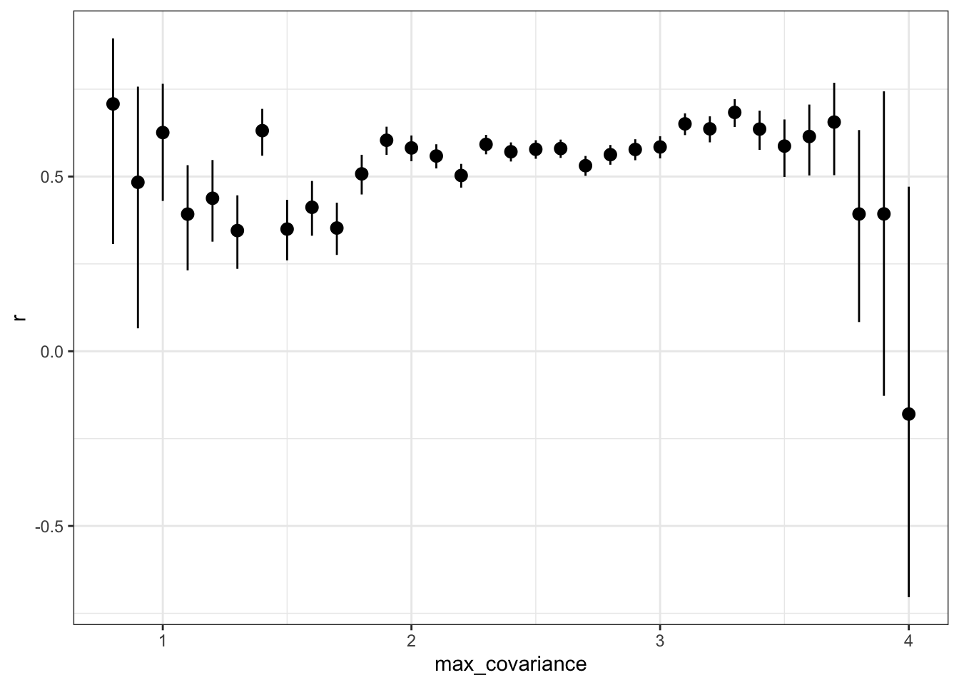

by_max_cov%>% 
  filter(max_covariance >= 2) %>% 
  summarise(broom::tidy(cor.test(synthetic_r, empirical_r)), sd_emp_r = sd(empirical_r), n = n()) %>% 
  kable(digits = 2, caption = "Accuracy for items with a maximal potential covariance (product of SDs) of at least 2")

Accuracy for items with a maximal potential covariance (product of SDs) of at least 2

estimate	statistic	p.value	parameter	conf.low	conf.high	method	alternative	sd_emp_r	n
0.58	114.91	0	26169	0.57	0.59	Pearson’s product-moment correlation	two.sided	0.23	26171

Is the accuracy lower for the pre-trained model?

ggplot(pt_rr_validation_llm, aes(synthetic_r, empirical_r, 
              ymin = empirical_r - empirical_r_se,
              ymax = empirical_r + empirical_r_se)) + 
  geom_abline(linetype = "dashed") +
  geom_point(color = "#00A0B0", alpha = 0.03, size = 1) +
  xlab("Synthetic inter-item correlation") + 
  ylab("Empirical inter-item correlation") +
  theme_bw() +
  coord_fixed(xlim = c(-1,1), ylim = c(-1,1)) -> pt_plot_items
pt_plot_items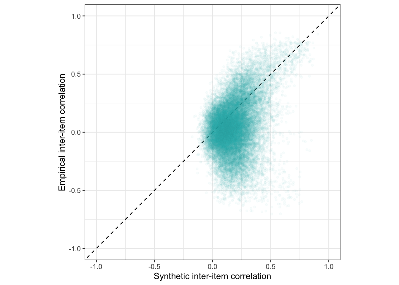

Averages

rr_validation_llm %>% summarise(
  mean(synthetic_r),
  mean(empirical_r),
  mean(abs(synthetic_r)),
  mean(abs(empirical_r)),
  prop_negative = sum(empirical_r < 0)/n(),
  prop_pos = sum(empirical_r > 0)/n(),
  `prop_below_-.10` = sum(empirical_r < -0.1)/n(),
  `prop_above_.10` = sum(empirical_r > 0.1)/n(),
) %>% kable(digits = 2, caption = "Average correlations")

Average correlations

mean(synthetic_r)	mean(empirical_r)	mean(abs(synthetic_r))	mean(abs(empirical_r))	prop_negative	prop_pos	prop_below_-.10	prop_above_.10
0.06	0.05	0.1	0.17	0.41	0.59	0.22	0.38

By sign & accuracy for absolute correlations

rr_validation_llm %>% 
  summarise(mean( sign(synthetic_r) > 0), mean( sign(empirical_r) > 0))

## # A tibble: 1 × 2
##   `mean(sign(synthetic_r) > 0)` `mean(sign(empirical_r) > 0)`
##                           <dbl>                         <dbl>
## 1                         0.673                         0.594

What if a human in the loop flipped the sign?

rr_validation_llm %>% filter(abs(synthetic_r) >= .10) %>% 
  group_by(sign(synthetic_r)) %>% 
  summarise(round(1 - mean(sign(empirical_r) == sign(synthetic_r)),2))

## # A tibble: 2 × 2
##   `sign(synthetic_r)` `round(1 - mean(sign(empirical_r) == sign(synthetic_r)), 2)`
##                 <dbl>                                                        <dbl>
## 1                  -1                                                         0.16
## 2                   1                                                         0.19

rr_validation_llm %>%  
  group_by(sign(synthetic_r)) %>% 
  summarise(round(1 - mean(sign(empirical_r) == sign(synthetic_r)),2))

## # A tibble: 2 × 2
##   `sign(synthetic_r)` `round(1 - mean(sign(empirical_r) == sign(synthetic_r)), 2)`
##                 <dbl>                                                        <dbl>
## 1                  -1                                                         0.37
## 2                   1                                                         0.3

cor_switch <- rr_validation_llm %>% mutate(synthetic_r = if_else(abs(synthetic_r) <= .10 | sign(synthetic_r) == sign(empirical_r), synthetic_r,
                                                                 -1*synthetic_r)) %>% 
  { broom::tidy(cor.test(.$synthetic_r, .$empirical_r)) }
cor_switch %>% select(accuracy = estimate, conf.low, conf.high) %>% mutate(kind = "manifest") %>% kable(caption = "If a human user flipped the sign to be correct for all synthetic estimates with an absolute magnitude bigger than .10", digits = 2)

If a human user flipped the sign to be correct for all synthetic estimates with an absolute magnitude bigger than .10

accuracy	conf.low	conf.high	kind
0.68	0.68	0.69	manifest

cor_abs <- broom::tidy(cor.test(abs(rr_validation_llm$synthetic_r), abs(rr_validation_llm$empirical_r)))
cor_neg <- rr_validation_llm %>% filter(empirical_r < 0) %>% 
 { broom::tidy(cor.test(.$synthetic_r, .$empirical_r)) }
cor_pos <- rr_validation_llm %>% filter(empirical_r > 0) %>% 
 { broom::tidy(cor.test(.$synthetic_r, .$empirical_r)) }

ggplot(rr_validation_llm, aes(abs(synthetic_r), abs(empirical_r), color = factor(sign(empirical_r)))) + 
  annotate("text", size = 3, x = 0, y = 0.98, vjust = 0, hjust = 0, label = with(cor_abs, { sprintf("accuracy absolute r = %.2f [%.2f;%.2f]", estimate, conf.low, conf.high) }), color = 'black') +
  annotate("text", size = 3, x = 0, y = 0.9, vjust = 0, hjust = 0, label = with(cor_neg, { sprintf("accuracy negative r = %.2f [%.2f;%.2f]", estimate, conf.low, conf.high) }), color = "#3366AA") +
  annotate("text", size = 3, x = 0, y = 0.82, vjust = 0, hjust = 0, label = with(cor_pos, { sprintf("accuracy positive r = %.2f [%.2f;%.2f]", estimate, conf.low, conf.high) }), color = "#00A0B0") +
  geom_abline(linetype = "dashed") +
  geom_point( alpha = 0.1, size = 1) +
  geom_smooth(method = "lm") +
  scale_color_manual("Sign of emp. r", values = c("1" = "#00A0B0", "-1" = "#3366AA")) +
  xlab("Absolute synthetic inter-item correlation") + 
  ylab("Absolute empirical inter-item correlation") +
  theme_bw() +
  coord_fixed(xlim = c(0,1), ylim = c(0,1)) -> abs_plot_items
abs_plot_items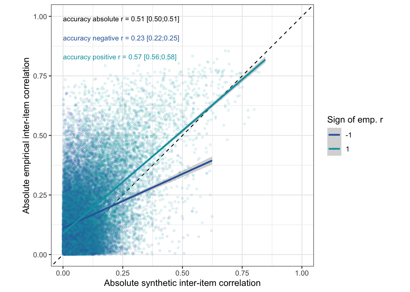

Does it matter how we define our exclusion criteria?

main_qs <- c("AAID", "PANAS", "PAQ", "PSS", "NEPS", "ULS", "FCV", "DAQ", "CESD", "HEXACO", "OCIR", "PTQ", "RAAS", "KSA", "SAS", "MFQ", "CQ", "OLBI", "UWES", "WGS")
rr_human_data_all = rio::import("data/processed/sosci_labelled_with_exclusion_criteria.rds")

manifest_and_latent_r <- function(data) {
  data <- data %>% 
    select(starts_with(main_qs)) %>% 
    select(-ends_with("_R")) %>% 
    longcor() %>% 
    left_join(rr_validation_llm %>% select(variable_1, variable_2, synthetic_r))
  se2 <- mean(data$empirical_r_se^2)
  model <- paste0('
    # Latent variables
    PearsonLatent =~ 1*empirical_r
  
    # Fixing error variances based on known standard errors
    empirical_r ~~ ',se2,'*empirical_r
  
    # Relationship between latent variables
    PearsonLatent ~~ synthetic_r
  ')

  fit <- sem(model, data = data)
  standardizedsolution(fit) %>% 
    filter(lhs == "PearsonLatent", rhs ==  "synthetic_r") %>% 
    mutate(model = "fine-tuned", kind = "latent outcome (SEM)") %>% 
    select(model, kind, accuracy = est.std, 
           conf.low = ci.lower, conf.high = ci.upper) %>% 
    bind_rows(
      broom::tidy(cor.test(data$empirical_r, data$synthetic_r)) %>% 
                    mutate(kind = "manifest") %>% 
        rename(accuracy = estimate) %>% 
        mutate(model = "fine-tuned")) %>% 
    mutate(`max N` = max(data$pairwise_n))
}


r_all <- rr_human_data_all %>% 
  manifest_and_latent_r() %>% 
  mutate(`exclusion criteria` = "No exclusions")

r_main <- rr_human_data_all %>% 
    mutate(time_per_item_outlier = time_per_item < 2,
                 even_odd_outlier = even_odd >= -.45,
                 psychsyn_outlier = psychsyn < 0.22,
                 psychant_outlier = psychant > -0.03,
                 mahal_outlier = careless::mahad(rr_human_data_all %>% select(starts_with(main_qs)), plot = FALSE, flag = TRUE, confidence = .99)$flagged) %>% 
    mutate(included = !not_serious & !time_per_item_outlier & 
             !even_odd_outlier & !psychsyn_outlier & !psychant_outlier & !mahal_flagged) %>% 
  filter(included) %>% 
  manifest_and_latent_r() %>% 
  mutate(`exclusion criteria` = "Adapted: <br>- exclude non-serious respondents<br>- item response time < 2s<br>- odd-even r <= .45<br>- psychometric synonym r < .22<br>- psychometric antonym r > -0.03<br>- Mahalanobis distance set for 99% specificity")

r_goldammer_1 <- rr_human_data_all %>% 
    mutate(time_per_item_outlier = time_per_item < 2,
                 even_odd_outlier = even_odd > -.30,
                 psychsyn_outlier = psychsyn < 0.22,
                 psychant_outlier = psychant > -0.03,
                 mahal_outlier = careless::mahad(rr_human_data_all %>% select(starts_with(main_qs)), plot = FALSE, flag = TRUE, confidence = .999)$flagged) %>% 
    mutate(included = !time_per_item_outlier & !even_odd_outlier & !psychsyn_outlier & !psychant_outlier & !mahal_flagged) %>% 
  filter(included) %>% 
  manifest_and_latent_r() %>% 
  mutate(`exclusion criteria` = "Goldammer heuristic: <br>- item response time < 2s<br>- odd-even r < .30<br>- psychometric synonym r < .22<br>- psychometric antonym r > -0.03<br>- Mahalanobis distance set for 999% specificity")

r_goldammer_2 <- rr_human_data_all %>% 
    mutate(time_per_item_outlier = time_per_item < 5.56,
                 even_odd_outlier = even_odd > -.42,
                 psychsyn_outlier = psychsyn < -0.03,
                 psychant_outlier = psychant > .36,
                 mahal_outlier = careless::mahad(rr_human_data_all %>% select(starts_with(main_qs)), plot = FALSE, flag = TRUE, confidence = .95)$flagged) %>% 
    mutate(included = !time_per_item_outlier & !even_odd_outlier & !psychsyn_outlier & !psychant_outlier & !mahal_flagged) %>% 
  filter(included) %>% 
  manifest_and_latent_r() %>% 
  mutate(`exclusion criteria` = "Goldammer 95% specificity: <br>- item response time < 5.56s<br>- odd-even r < .42<br>- psychometric synonym r < -0.03<br>- psychometric antonym r > .36<br>- Mahalanobis distance set for 95% specificity")


r_goldammer_3 <- rr_human_data_all %>% 
    mutate(time_per_item_outlier = time_per_item < 4.97,
                 even_odd_outlier = even_odd > -.26,
                 psychsyn_outlier = psychsyn < -0.30,
                 psychant_outlier = psychant > .55,
                 mahal_outlier = careless::mahad(rr_human_data_all %>% select(starts_with(main_qs)), plot = FALSE, flag = TRUE, confidence = .99)$flagged) %>% 
    mutate(included = !time_per_item_outlier & !even_odd_outlier & !psychsyn_outlier & !psychant_outlier & !mahal_flagged) %>% 
  filter(included) %>% 
  manifest_and_latent_r() %>% 
  mutate(`exclusion criteria` = "Goldammer 99% specificity: <br>- item response time < 5.56s<br>- odd-even r < .42<br>- psychometric synonym r < -0.03<br>- psychometric antonym r > .36<br>- Mahalanobis distance set for 99% specificity")

    
r_strict_reading_of_prereg <- rr_human_data_all %>% 
    mutate(psychsyn_outlier = psychsyn < 0.6,
      psychant_outlier = psychant > -0.4,
      not_us_citizen = Nationality != "United States"
      ) %>%
    filter(if_all(c(longstring_outlier, `mahal_dist_outlier_.5`, psychsyn_outlier, psychant_outlier, even_odd_outlier, not_us_citizen), ~ . == FALSE)) %>%
  manifest_and_latent_r() %>% 
  mutate(`exclusion criteria` = "Strict preregistered criteria: <br>- odd-even r < mean + 0.2 * SD<br>- psychometric synonym r < .60<br>- psychometric antonym r > -0.40<br>- Mahalanobis distance < mean + 0.5 * SD<br>-Not US citizen")


r_main_first_450 <- rr_human_data_all %>% 
    mutate(mahal_outlier = careless::mahad(rr_human_data_all %>% select(starts_with(main_qs)), plot = FALSE, flag = TRUE, confidence = .99)$flagged) %>% 
  arrange(`Completed at`) %>% 
  filter(row_number () <= 450) %>% 
    mutate(time_per_item_outlier = time_per_item < 2,
                 even_odd_outlier = even_odd >= -.45,
                 psychsyn_outlier = psychsyn < 0.22,
                 psychant_outlier = psychant > -0.03) %>% 
    mutate(included = !not_serious & !time_per_item_outlier & 
             !even_odd_outlier & !psychsyn_outlier & !psychant_outlier & !mahal_flagged) %>% 
  filter(included) %>% 
  manifest_and_latent_r() %>% 
  mutate(`exclusion criteria` = "Adapted + Prereg N: <br>- the adapted criteria<br>- Only the first 450 participants, our preregistered sample size.")


r_main_us <- rr_human_data_all %>% 
    mutate(time_per_item_outlier = time_per_item < 2,
                 even_odd_outlier = even_odd >= -.45,
                 psychsyn_outlier = psychsyn < 0.22,
                 psychant_outlier = psychant > -0.03,
                 mahal_outlier = careless::mahad(rr_human_data_all %>% select(starts_with(main_qs)), plot = FALSE, flag = TRUE, confidence = .99)$flagged,
                 us_citizen = Nationality == "United States",
                 english_first_language = Language == "English") %>% 
    mutate(included = !not_serious & !time_per_item_outlier & 
             !even_odd_outlier & !psychsyn_outlier & !psychant_outlier & !mahal_flagged & us_citizen & english_first_language) %>% 
  filter(included) %>% 
  manifest_and_latent_r() %>% 
  mutate(`exclusion criteria` = "Adapted + US English: <br>- the adapted criteria<br>- US citizens, not just residents,- English first language")

r_main_approvals <- rr_human_data_all %>% 
    mutate(time_per_item_outlier = time_per_item < 2,
                 even_odd_outlier = even_odd >= -.45,
                 psychsyn_outlier = psychsyn < 0.22,
                 psychant_outlier = psychant > -0.03,
                 mahal_outlier = careless::mahad(rr_human_data_all %>% select(starts_with(main_qs)), plot = FALSE, flag = TRUE, confidence = .99)$flagged,
                 us_citizen = Nationality == "United States",
                 more_than_20_approvals = `Total approvals` > 20,
                 english_first_language = Language == "English") %>% 
    mutate(included = !not_serious & !time_per_item_outlier & 
             !even_odd_outlier & !psychsyn_outlier & !psychant_outlier & !mahal_flagged & us_citizen & more_than_20_approvals) %>% 
  filter(included) %>% 
  manifest_and_latent_r() %>% 
  mutate(`exclusion criteria` = "Adapted + US + > 20 approvals: <br>- the adapted criteria<br>- US citizens, not just residents,- More than 20 approvals")


r_adapted_reading_of_prereg <- rr_human_data_all %>% 
    mutate(psychsyn_outlier = psychsyn < 0.22,
      psychant_outlier = psychant > -0.03) %>%
    filter(if_all(c(`mahal_dist_outlier_.5`, psychsyn_outlier, psychant_outlier, even_odd_outlier), ~ . == FALSE)) %>%
  manifest_and_latent_r() %>% 
  mutate(`exclusion criteria` = "Corrected prereg criteria:<br>- odd-even r < mean + 0.2 * SD,<br>- psychometric synonym r < .22,<br> - psychometric antonym r > -0.03, <br>- Mahalanobis distance < mean + 0.5 * SD")

The manifest accuracy is expected to decrease slightly with sample size because it is attenuated by sampling error in the empirical correlations. The latent accuracy should only grow more uncertain with decreased sample size.

exclusion_criteria <- bind_rows(
  r_all, r_main, r_strict_reading_of_prereg, r_adapted_reading_of_prereg, 
  r_goldammer_1, r_goldammer_2, r_goldammer_3, r_main_us, r_main_approvals,
  r_main_first_450
  )
exclusion_criteria %>% 
    select(`exclusion criteria`, model, kind, accuracy, conf.low, conf.high, `max N`) %>% 
  knitr::kable(digits = 2, caption = "Accuracy when human data is filtered by different exclusion criteria", format = "markdown")

Accuracy when human data is filtered by different exclusion criteria

exclusion criteria	model	kind	accuracy	conf.low	conf.high	max N
No exclusions	fine-tuned	latent outcome (SEM)	0.59	0.58	0.59	470
No exclusions	fine-tuned	manifest	0.57	0.56	0.58	470
Adapted: - exclude non-serious respondents - item response time < 2s - odd-even r <= .45 - psychometric synonym r < .22 - psychometric antonym r > -0.03 - Mahalanobis distance set for 99% specificity	fine-tuned	latent outcome (SEM)	0.58	0.58	0.59	336
Adapted: - exclude non-serious respondents - item response time < 2s - odd-even r <= .45 - psychometric synonym r < .22 - psychometric antonym r > -0.03 - Mahalanobis distance set for 99% specificity	fine-tuned	manifest	0.57	0.56	0.58	336
Strict preregistered criteria: - odd-even r < mean + 0.2 * SD - psychometric synonym r < .60 - psychometric antonym r > -0.40 - Mahalanobis distance < mean + 0.5 * SD -Not US citizen	fine-tuned	latent outcome (SEM)	0.57	0.56	0.58	116
Strict preregistered criteria: - odd-even r < mean + 0.2 * SD - psychometric synonym r < .60 - psychometric antonym r > -0.40 - Mahalanobis distance < mean + 0.5 * SD -Not US citizen	fine-tuned	manifest	0.54	0.53	0.54	116
Corrected prereg criteria: - odd-even r < mean + 0.2 * SD, - psychometric synonym r < .22, - psychometric antonym r > -0.03, - Mahalanobis distance < mean + 0.5 * SD	fine-tuned	latent outcome (SEM)	0.58	0.58	0.59	291
Corrected prereg criteria: - odd-even r < mean + 0.2 * SD, - psychometric synonym r < .22, - psychometric antonym r > -0.03, - Mahalanobis distance < mean + 0.5 * SD	fine-tuned	manifest	0.57	0.56	0.57	291
Goldammer heuristic: - item response time < 2s - odd-even r < .30 - psychometric synonym r < .22 - psychometric antonym r > -0.03 - Mahalanobis distance set for 999% specificity	fine-tuned	latent outcome (SEM)	0.58	0.58	0.59	341
Goldammer heuristic: - item response time < 2s - odd-even r < .30 - psychometric synonym r < .22 - psychometric antonym r > -0.03 - Mahalanobis distance set for 999% specificity	fine-tuned	manifest	0.57	0.56	0.58	341
Goldammer 95% specificity: - item response time < 5.56s - odd-even r < .42 - psychometric synonym r < -0.03 - psychometric antonym r > .36 - Mahalanobis distance set for 95% specificity	fine-tuned	latent outcome (SEM)	0.58	0.58	0.59	143
Goldammer 95% specificity: - item response time < 5.56s - odd-even r < .42 - psychometric synonym r < -0.03 - psychometric antonym r > .36 - Mahalanobis distance set for 95% specificity	fine-tuned	manifest	0.54	0.53	0.55	143
Goldammer 99% specificity: - item response time < 5.56s - odd-even r < .42 - psychometric synonym r < -0.03 - psychometric antonym r > .36 - Mahalanobis distance set for 99% specificity	fine-tuned	latent outcome (SEM)	0.58	0.57	0.59	185
Goldammer 99% specificity: - item response time < 5.56s - odd-even r < .42 - psychometric synonym r < -0.03 - psychometric antonym r > .36 - Mahalanobis distance set for 99% specificity	fine-tuned	manifest	0.55	0.54	0.55	185
Adapted + US English: - the adapted criteria - US citizens, not just residents,- English first language	fine-tuned	latent outcome (SEM)	0.58	0.57	0.59	284
Adapted + US English: - the adapted criteria - US citizens, not just residents,- English first language	fine-tuned	manifest	0.56	0.56	0.57	284
Adapted + US + > 20 approvals: - the adapted criteria - US citizens, not just residents,- More than 20 approvals	fine-tuned	latent outcome (SEM)	0.59	0.58	0.59	284
Adapted + US + > 20 approvals: - the adapted criteria - US citizens, not just residents,- More than 20 approvals	fine-tuned	manifest	0.57	0.56	0.57	284
Adapted + Prereg N: - the adapted criteria - Only the first 450 participants, our preregistered sample size.	fine-tuned	latent outcome (SEM)	0.58	0.58	0.59	325
Adapted + Prereg N: - the adapted criteria - Only the first 450 participants, our preregistered sample size.	fine-tuned	manifest	0.57	0.56	0.58	325

exclusion_criteria %>% 
  mutate(`exclusion criteria` = fct_rev(fct_inorder(str_c(str_sub(`exclusion criteria`, 1, coalesce(str_locate(`exclusion criteria`, ":")[, 1]-1, -1)),", n=", `max N`)))) %>% 
ggplot(aes(x = `exclusion criteria`, accuracy, ymin = conf.low, ymax = conf.high, color = kind)) +
  geom_pointrange() + 
  scale_color_viridis_d(end = 0.7) +
  geom_text(aes(label = sprintf("%.2f", accuracy)), vjust = -1) +
  coord_flip()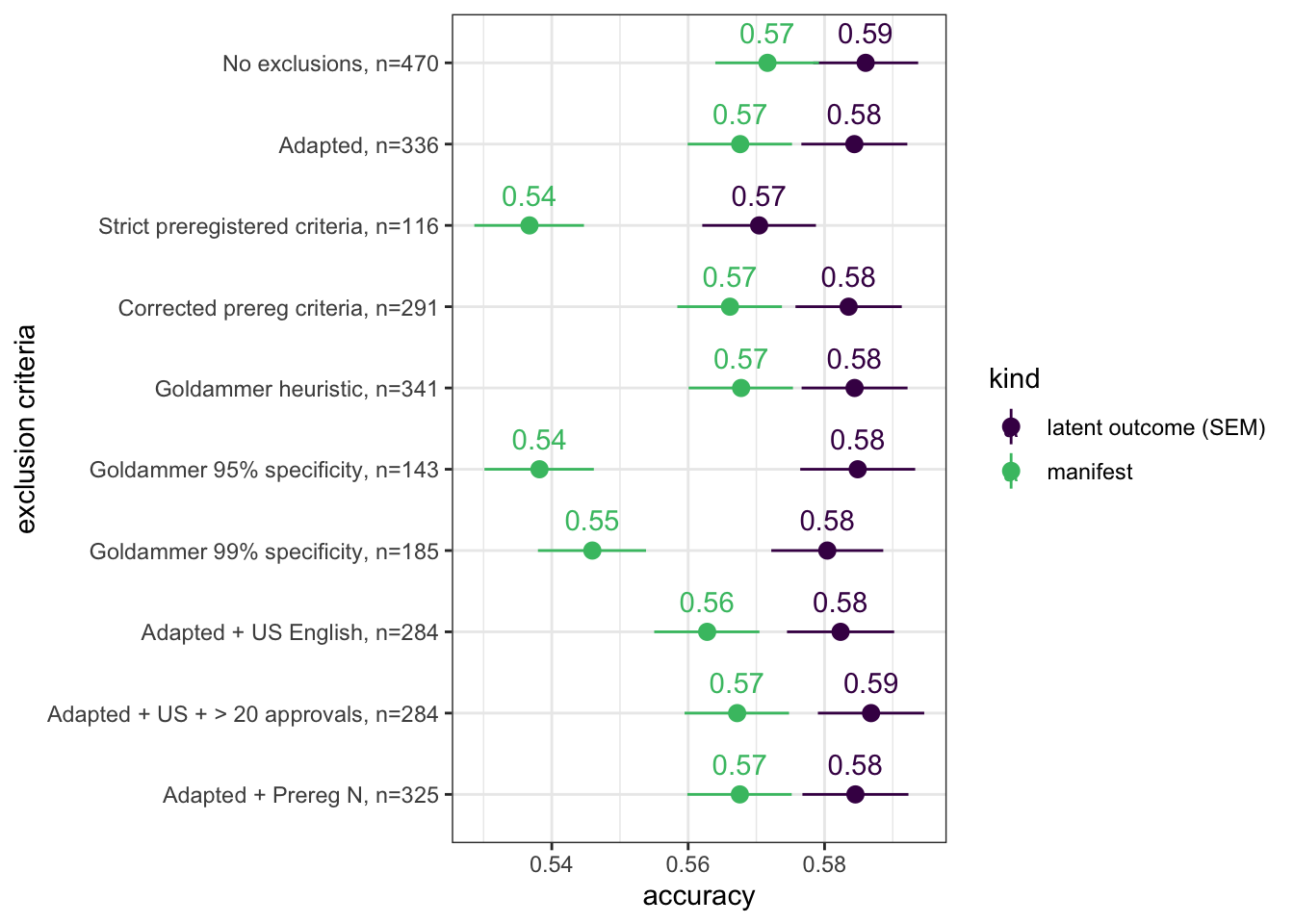

Consequences of data leakage

Below, we import our search results of the SBERT training corpus. We identify validation study items with matches, investigate these matches and tabulate accuracy without potentially leaked items.

leaked <- rio::import("data/intermediate/search_results.parquet") %>% 
  mutate(item_text = str_to_lower(item_text))
leaked_items <- leaked %>% group_by(item_text) %>% summarise(n = n())


item_pair_table_l <- item_pair_table_numeric %>% 
  mutate(item_text_1l = str_to_lower(item_text_1),
         item_text_2l = str_to_lower(item_text_2))

items <- bind_rows(item_pair_table_l %>% select(Instrument = InstrumentA, item_textl = item_text_1l),
                   item_pair_table_l %>% select(Instrument = InstrumentB, item_textl = item_text_2l)) %>% 
  distinct()

# items %>% inner_join(leaked, by = c("item_textl" = "item_text")) %>% View

leaked_items_validation <- leaked_items %>% right_join(
  items, by = c("item_text" = "item_textl")) %>% 
  mutate(length = str_length(item_text),
         n = coalesce(n, 0))

leaked_items_validation %>% group_by(Instrument) %>% 
  summarise(leaked = sum(n>0), items = n(), percentage = sum(n>0)/n()*100, matches = sum(n)) %>% 
  arrange(percentage) %>% 
  kable(caption = "Number and percent of items leaked per instrument", digits = 0)

Number and percent of items leaked per instrument

Instrument	leaked	items	percentage	matches
Attitudes Toward AI in Defense Scale	0	6	0	0
Authoritarianism Short Scale	0	9	0	0
Chronotype Questionnaire	0	16	0	0
Disgust Avoidance Questionnaire	0	17	0	0
Fear of COVID-19 Scale	0	7	0	0
HEXACO-60	0	30	0	0
Obsessive–Compulsive Inventory (Revised)	0	18	0	0
Oldenburg Burnout Inventory (English Translation)	0	8	0	0
Perseverative Thinking Questionnaire	0	15	0	0
Perth Alexithymia Questionnaire	0	10	0	0
Positive and Negative Affect Schedule	0	8	0	0
Revised Adult Attachment Scale	0	11	0	0
Survey Attitude Scale	0	9	0	0
Work Gratitude Scale	0	10	0	0
Perceived Stress Scale	1	14	7	1
UCLA Loneliness Scale (Short Form)	1	8	12	13
Moral Foundations Questionnaire	2	11	18	2
Center for Epidemiological Studies Depression Scale	7	20	35	885
New Ecological Paradigm Scale	5	10	50	7
Utrecht Work Engagement Scale (Short Version)	8	9	89	64

rr_validation_llm_leakage <- item_pair_table_l %>% 
  left_join(leaked_items_validation %>% rename(n_1 = n, item_text_1l = item_text), by = "item_text_1l") %>% 
  left_join(leaked_items_validation %>% rename(n_2 = n, item_text_2l = item_text), by = "item_text_2l")

rr_validation_llm_leakage %>% 
  group_by(possibly_leaked_instrument = str_detect(InstrumentA, "(New Ecological|Utrecht Work)") |
             str_detect(InstrumentB, "(New Ecological|Utrecht Work)")) %>% 
  summarise(broom::tidy(cor.test(synthetic_r, empirical_r)), pt_cor = cor(pt_synthetic_r, empirical_r), rmse = sqrt(mean((empirical_r - synthetic_r)^2)), pt_rmse = sqrt(mean((empirical_r - pt_synthetic_r)^2)), n = n()) %>% 
  select(possibly_leaked_instrument, r = estimate, conf.low, conf.high, pt_cor, rmse, pt_rmse, n) %>% 
  arrange(r) %>% 
  kable(caption = "Accuracy by whether the instrument plausibly leaked (>=50% items found in corpus)", digits = 2)

Accuracy by whether the instrument plausibly leaked (>=50% items found in corpus)

possibly_leaked_instrument	r	conf.low	conf.high	pt_cor	rmse	pt_rmse	n
FALSE	0.57	0.56	0.58	0.30	0.19	0.26	25651
TRUE	0.59	0.57	0.61	0.29	0.16	0.24	4484

rr_validation_llm_leakage %>% 
  group_by(occurred = n_1 > 0 | n_2 > 0) %>% 
  summarise(broom::tidy(cor.test(synthetic_r, empirical_r)), pt_cor = cor(pt_synthetic_r, empirical_r), rmse = sqrt(mean((empirical_r - synthetic_r)^2)), pt_rmse = sqrt(mean((empirical_r - pt_synthetic_r)^2)), n = n()) %>% 
  select(occurred, r = estimate, conf.low, conf.high, pt_cor, rmse, pt_rmse, n) %>% 
  arrange(r) %>% 
  kable(caption = "Accuracy by whether the item occurred in corpus (including trivially short items)", digits = 2)

Accuracy by whether the item occurred in corpus (including trivially short items)

occurred	r	conf.low	conf.high	pt_cor	rmse	pt_rmse	n
FALSE	0.53	0.52	0.54	0.29	0.18	0.25	24531
TRUE	0.69	0.67	0.70	0.35	0.19	0.28	5604

Full table

Full table of synthetic and empirical item pair correlations

Synthetic Reliabilities

scales <- readRDS(file = file.path(data_path, glue("scales_with_alpha_se_rr.rds")))
real_scales <- scales %>% filter(type == "real")
scales <- scales %>% filter(number_of_items >= 3)

Accuracy

se2 <- mean(scales$empirical_alpha_se^2)
r <- broom::tidy(cor.test(scales$empirical_alpha, scales$synthetic_alpha))
pt_r <- broom::tidy(cor.test(scales$empirical_alpha, scales$pt_synthetic_alpha))

model <- paste0('
  # Latent variables
  latent_real_rel =~ 1*empirical_alpha

  # Fixing error variances based on known standard errors
  empirical_alpha ~~ ',se2,'*empirical_alpha

  # Relationship between latent variables
  latent_real_rel ~~ synthetic_alpha
')

fit <- sem(model, data = scales)
pt_fit <- sem(model, data = scales %>% 
                select(empirical_alpha, synthetic_alpha = pt_synthetic_alpha))

# Bayesian EIV PT
pt_m_lmsynth_rel_scales <- brm(
  bf(empirical_alpha | mi(empirical_alpha_se) ~ synthetic_alpha,
     sigma ~ s(synthetic_alpha)), data = scales %>% 
                select(empirical_alpha, synthetic_alpha = pt_synthetic_alpha, empirical_alpha_se), 
  file = "ignore/pt_m_synth_rr_rel_lm")

newdata <- pt_m_lmsynth_rel_scales$data %>% select(empirical_alpha, synthetic_alpha, empirical_alpha_se)
epreds <- epred_draws(newdata = newdata, obj = pt_m_lmsynth_rel_scales, re_formula = NA)
preds <- predicted_draws(newdata = newdata, obj = pt_m_lmsynth_rel_scales, re_formula = NA)
epred_preds <- epreds %>% left_join(preds)
by_draw <- epred_preds %>% group_by(.draw) %>% 
  summarise(.epred = var(.epred),
            .prediction = var(.prediction),
            sigma = sqrt(.prediction - .epred),
            latent_r = sqrt(.epred/.prediction))

pt_accuracy_bayes_rels <- by_draw %>% mean_hdci(latent_r)

# Bayesian EIV FT
m_lmsynth_rel_scales <- brm(
  bf(empirical_alpha | mi(empirical_alpha_se) ~ synthetic_alpha,
     sigma ~ s(synthetic_alpha)), data = scales, 
  iter = 6000, 
  file = "ignore/m_synth_rr_rel_lm")

newdata <- m_lmsynth_rel_scales$data %>% select(empirical_alpha, synthetic_alpha, empirical_alpha_se)
epreds <- epred_draws(newdata = newdata, obj = m_lmsynth_rel_scales, re_formula = NA)
preds <- predicted_draws(newdata = newdata, obj = m_lmsynth_rel_scales, re_formula = NA)
epred_preds <- epreds %>% left_join(preds)
by_draw <- epred_preds %>% group_by(.draw) %>% 
  summarise(
             mae = mean(abs(.epred - .prediction)),
            .epred = var(.epred),
            .prediction = var(.prediction),
            sigma = sqrt(.prediction - .epred),
            latent_r = sqrt(.epred/.prediction))

accuracy_bayes_rels <- by_draw %>% mean_hdci(latent_r)

bind_rows(
  pt_r %>% 
    mutate(model = "pre-trained", kind = "manifest") %>% 
    select(model, kind, accuracy = estimate, conf.low, conf.high),
  standardizedsolution(pt_fit) %>% 
    filter(lhs == "latent_real_rel", rhs ==  "synthetic_alpha") %>% 
    mutate(model = "pre-trained", kind = "latent outcome (SEM)") %>% 
    select(model, kind, accuracy = est.std, 
           conf.low = ci.lower, conf.high = ci.upper),
  pt_accuracy_bayes_rels %>% 
      mutate(model = "pre-trained", kind = "latent outcome (Bayesian EIV)") %>% 
      select(model, kind, accuracy = latent_r, conf.low = .lower, conf.high = .upper),
  r %>% 
    mutate(model = "fine-tuned", kind = "manifest") %>% 
    select(model, kind, accuracy = estimate, conf.low, conf.high),
  standardizedsolution(fit) %>% 
    filter(lhs == "latent_real_rel", rhs ==  "synthetic_alpha") %>% 
    mutate(model = "fine-tuned", kind = "latent outcome (SEM)") %>% 
    select(model, kind, accuracy = est.std, 
           conf.low = ci.lower, conf.high = ci.upper),
  accuracy_bayes_rels %>% 
    mutate(model = "fine-tuned", kind = "latent outcome (Bayesian EIV)") %>% 
    select(model, kind, accuracy = latent_r, conf.low = .lower, conf.high = .upper)
  ) %>% 
  kable(digits = 2, caption = "Accuracy across language models and methods")

Accuracy across language models and methods

model	kind	accuracy	conf.low	conf.high
pre-trained	manifest	0.64	0.56	0.71
pre-trained	latent outcome (SEM)	0.65	0.58	0.73
pre-trained	latent outcome (Bayesian EIV)	0.70	0.61	0.79
fine-tuned	manifest	0.85	0.81	0.88
fine-tuned	latent outcome (SEM)	0.86	0.83	0.90
fine-tuned	latent outcome (Bayesian EIV)	0.84	0.79	0.90

Prediction error plot according to synthetic estimate

m_lmsynth_rel_scales

##  Family: gaussian
##   Links: mu = identity; sigma = log
## Formula: empirical_alpha | mi(empirical_alpha_se) ~ synthetic_alpha
##          sigma ~ s(synthetic_alpha)
##    Data: scales (Number of observations: 257)
##   Draws: 4 chains, each with iter = 6000; warmup = 3000; thin = 1;
##          total post-warmup draws = 12000
##
## Smooth Terms:
##                               Estimate Est.Error l-95% CI u-95% CI Rhat Bulk_ESS Tail_ESS
## sds(sigma_ssynthetic_alpha_1)     3.53      1.68     1.12     7.57 1.00     1756     1034
##
## Population-Level Effects:
##                          Estimate Est.Error l-95% CI u-95% CI Rhat Bulk_ESS Tail_ESS
## Intercept                   -0.02      0.02    -0.05     0.02 1.00     7806     7356
## sigma_Intercept             -1.44      0.05    -1.54    -1.34 1.00     8401     7731
## synthetic_alpha              1.15      0.03     1.09     1.22 1.00     4029     1530
## sigma_ssynthetic_alpha_1     1.28      6.46    -8.91    15.77 1.00     1524      574
##
## Draws were sampled using sample(hmc). For each parameter, Bulk_ESS
## and Tail_ESS are effective sample size measures, and Rhat is the potential
## scale reduction factor on split chains (at convergence, Rhat = 1).

kable(rmse_alpha <- by_draw %>% mean_hdci(sigma), caption = "Average prediction error (RMSE)", digits = 2)

Average prediction error (RMSE)

sigma	.lower	.upper	.width	.point	.interval
0.27	0.21	0.33	0.95	mean	hdci

kable(mae_alpha <- by_draw %>% mean_hdci(mae), caption = "Average prediction error (MAE)", digits = 2)

Average prediction error (MAE)

mae	.lower	.upper	.width	.point	.interval
0.21	0.18	0.24	0.95	mean	hdci

plot_prediction_error_alpha <- plot(conditional_effects(m_lmsynth_rel_scales, dpar = "sigma"), plot = F)[[1]] + 
  theme_bw() + 
  geom_smooth(stat = "identity", color = "#a48500", fill = "#EDC951") + 
  xlab("Synthetic Cronbach's alpha") + 
  ylab("Prediction error (sigma)") +
  coord_cartesian(xlim = c(-1, 1), ylim = c(0, 0.35))
plot_prediction_error_alpha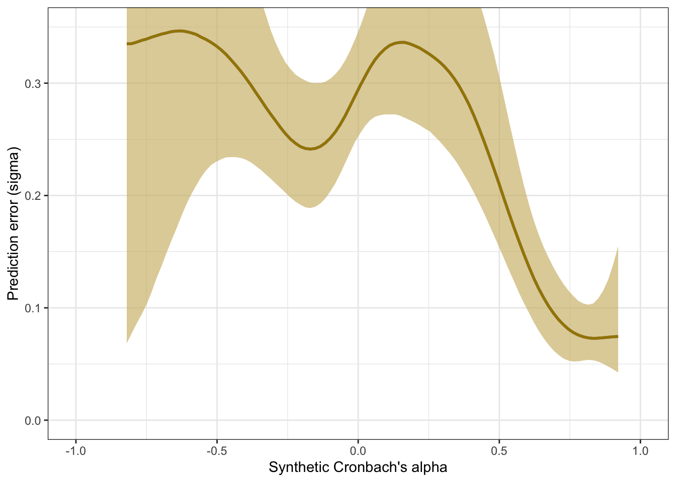

Scatter plot

pred <- conditional_effects(m_lmsynth_rel_scales, method = "predict")
ggplot(scales, aes(synthetic_alpha, empirical_alpha, 
                   color = str_detect(scale, "^random"), 
              ymin = empirical_alpha - empirical_alpha_se,
              ymax = empirical_alpha + empirical_alpha_se)) + 
  geom_abline(linetype = "dashed") +
  geom_point(alpha = 0.6, size = 1) +
  geom_smooth(aes(
    x = synthetic_alpha,
    y = estimate__,
    ymin = lower__,
    ymax = upper__,
  ), stat = "identity", 
  color = "#a48500",
  fill = "#EDC951",
  data = as.data.frame(pred$synthetic_alpha)) +
  scale_color_manual(values = c("#00A0B0", "#6A4A3C"),
                     guide = "none") +
  xlab("Synthetic Cronbach's alpha") + 
  ylab("Empirical Cronbach's alpha") +
  theme_bw() +
  coord_fixed(xlim = c(-1, 1), ylim = c(-1,1))  -> plot_rels
plot_rels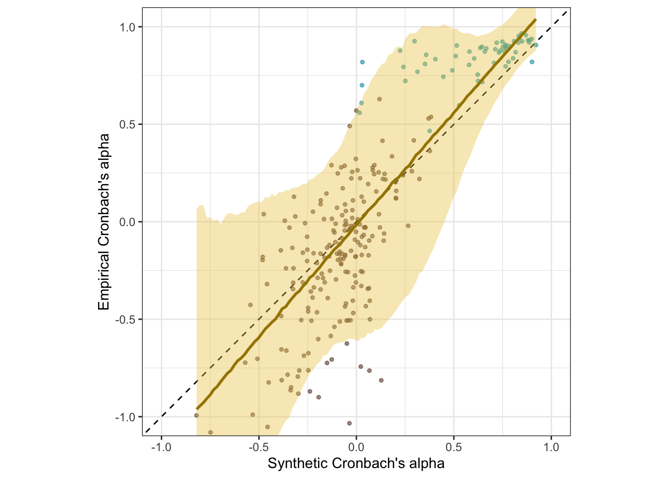

Interactive plot

(scales %>% 
  filter(!str_detect(scale, "^random")) %>%
  mutate(synthetic_alpha = round(synthetic_alpha, 2),
         empirical_alpha = round(empirical_alpha, 2),
         scale = str_replace_all(scale, "_+", " ")) %>% 
ggplot(., aes(synthetic_alpha, empirical_alpha, 
              # ymin = empirical_r - empirical_r_se, 
              # ymax = empirical_r + empirical_r_se, 
              label = scale)) + 
  geom_abline(linetype = "dashed") +
  geom_point(alpha = 0.3, size = 1, color = "#00A0B0") +
  xlab("Synthetic Cronbach's alpha") + 
  ylab("Empirical Cronbach's alpha") +
  theme_bw() +
  theme(legend.position='none') + 
   coord_fixed(xlim = c(-1,1), ylim = c(-1,1))) %>% 
  ggplotly()

Table

scales %>% 
  filter(type != "random") %>% 
  mutate(empirical_alpha = sprintf("%.2f±%.3f", empirical_alpha,
                               empirical_alpha_se),
         synthetic_alpha = sprintf("%.2f", synthetic_alpha),
         scale = str_replace_all(scale, "_+", " ")
         ) %>% 
  select(scale, empirical_alpha, synthetic_alpha, number_of_items) %>% 
  DT::datatable(rownames = FALSE,
                filter = "top")

Robustness checks

Accuracy by whether scales were real or random

The SurveyBot3000 does not “know” whether scales were published in the literature or formed at random. Knowing what we do about the research literature in psychology, we can infer that published scales will usually exceed the Nunnally threshold of .70. Hence, we know that the synthetic alphas for published scales should rarely be below .70. If we regress synthetic alphas on empirical alphas separately for the scales taken from the literature, we see this as a bias (a positive regression intercept of .68 and a slope ≠ 1, .26). Still, the synthetic alpha estimates are predictive of empirical alphas with an accuracy of .65.

There is no clear bias for the random scales. When both are analyzed jointly, the clear selection bias for the published scales is mostly averaged out but is reflected in the slope exceeding 1.

scales %>% 
  group_by(type) %>% 
  summarise(broom::tidy(cor.test(synthetic_alpha, empirical_alpha)), sd_alpha = sd(empirical_alpha), n = n()) %>% 
  knitr::kable(digits = 2, caption = "Accuracy shown separately for randomly formed and real scales")

Accuracy shown separately for randomly formed and real scales

type	estimate	statistic	p.value	parameter	conf.low	conf.high	method	alternative	sd_alpha	n
random	0.63	11.47	0	198	0.54	0.71	Pearson’s product-moment correlation	two.sided	0.37	200
real	0.64	6.11	0	55	0.45	0.77	Pearson’s product-moment correlation	two.sided	0.10	57

scales %>% 
  group_by(type) %>% 
  summarise(broom::tidy(lm(empirical_alpha ~ synthetic_alpha)), n = n()) %>% 
  knitr::kable(digits = 2, caption = "Regression intercepts and slopes for randomly formed and real scales")

Regression intercepts and slopes for randomly formed and real scales

type	term	estimate	std.error	statistic	p.value	n
random	(Intercept)	-0.08	0.02	-3.44	0	200
random	synthetic_alpha	1.15	0.10	11.47	0	200
real	(Intercept)	0.68	0.03	23.76	0	57
real	synthetic_alpha	0.26	0.04	6.11	0	57

As in our Stage 1 submission

Here are the results if we calculate the accuracy and prediction error as in the Stage 1 submission. We now think this approach, by conditioning on random variation in the empirical correlations, gave a misleading picture of the accuracy and bias of the synthetic Cronbach’s alphas. Here we report the results if we conduct the analysis as in Stage 1 (but with the corrected SE of empirical alphas).

s1_scales <- scales %>%
  filter(number_of_items > 2) %>% 
  rowwise() %>%
  mutate(reverse_items = if_else(type == "random", list(reverse_items_by_1st), list(reverse_items)),
         r_real_rev = list(reverse_items(r_real, reverse_items)),
         pt_r_llm_rev = list(reverse_items(pt_r_llm, reverse_items)),
         r_llm_rev = list(reverse_items(r_llm, reverse_items))) %>%
  mutate(
    rel_real = list(psych::alpha(r_real_rev, keys = F, n.obs = N)$feldt),
    rel_llm = list(psych::alpha(r_llm_rev, keys = F, n.obs = N)$feldt),
    rel_pt_llm = list(psych::alpha(pt_r_llm_rev, keys = F, n.obs = N)$feldt)) %>%
  mutate(empirical_alpha = rel_real$alpha$raw_alpha,
         synthetic_alpha = rel_llm$alpha$raw_alpha,
         pt_synthetic_alpha = rel_pt_llm$alpha$raw_alpha) %>%
  mutate(
    empirical_alpha_se = mean(diff(unlist(psychometric::alpha.CI(empirical_alpha, k = number_of_items, N = N, level = 0.95))))/1.96) %>% 
      filter(empirical_alpha > 0)

s1_r <- broom::tidy(cor.test(s1_scales$empirical_alpha, s1_scales$synthetic_alpha))

m_lmsynth_rel_scales_s1 <- brm(
  bf(empirical_alpha | mi(empirical_alpha_se) ~ synthetic_alpha,
     sigma ~ poly(synthetic_alpha, degree = 3)), data = s1_scales, 
  iter = 6000, control = list(adapt_delta = 0.9),
  file = "ignore/m_synth_rr_rel_lm_as_stage_1")

pred <- conditional_effects(m_lmsynth_rel_scales_s1, method = "predict")
ggplot(s1_scales, aes(synthetic_alpha, empirical_alpha, 
                   color = str_detect(scale, "^random"), 
              ymin = empirical_alpha - empirical_alpha_se,
              ymax = empirical_alpha + empirical_alpha_se)) + 
  geom_abline(linetype = "dashed") +
  geom_point(alpha = 0.6, size = 1) +
  geom_smooth(aes(
    x = synthetic_alpha,
    y = estimate__,
    ymin = lower__,
    ymax = upper__,
  ), stat = "identity", 
  color = "#a48500",
  fill = "#EDC951",
  data = as.data.frame(pred$synthetic_alpha)) +  scale_color_manual(values = c("#00A0B0", "#6A4A3C"),
                     guide = "none") +
  xlab("Synthetic Cronbach's alpha") + 
  ylab("Empirical Cronbach's alpha") +
  theme_bw() +
  coord_fixed(xlim = c(-1, 1), ylim = c(-1,1))  -> s1_plot_rels

newdata <- m_lmsynth_rel_scales_s1$data %>% select(empirical_alpha, synthetic_alpha, empirical_alpha_se)
epreds <- epred_draws(newdata = newdata, obj = m_lmsynth_rel_scales_s1, re_formula = NA)
preds <- predicted_draws(newdata = newdata, obj = m_lmsynth_rel_scales_s1, re_formula = NA)
epred_preds <- epreds %>% left_join(preds)
by_draw <- epred_preds %>% group_by(.draw) %>% 
  summarise(
             mae = mean(abs(.epred - .prediction)),
            .epred = var(.epred),
            .prediction = var(.prediction),
            sigma = sqrt(.prediction - .epred),
            latent_r = sqrt(.epred/.prediction))

accuracy_bayes_rels_poly <- by_draw %>% mean_hdci(latent_r)

s1_plot_rels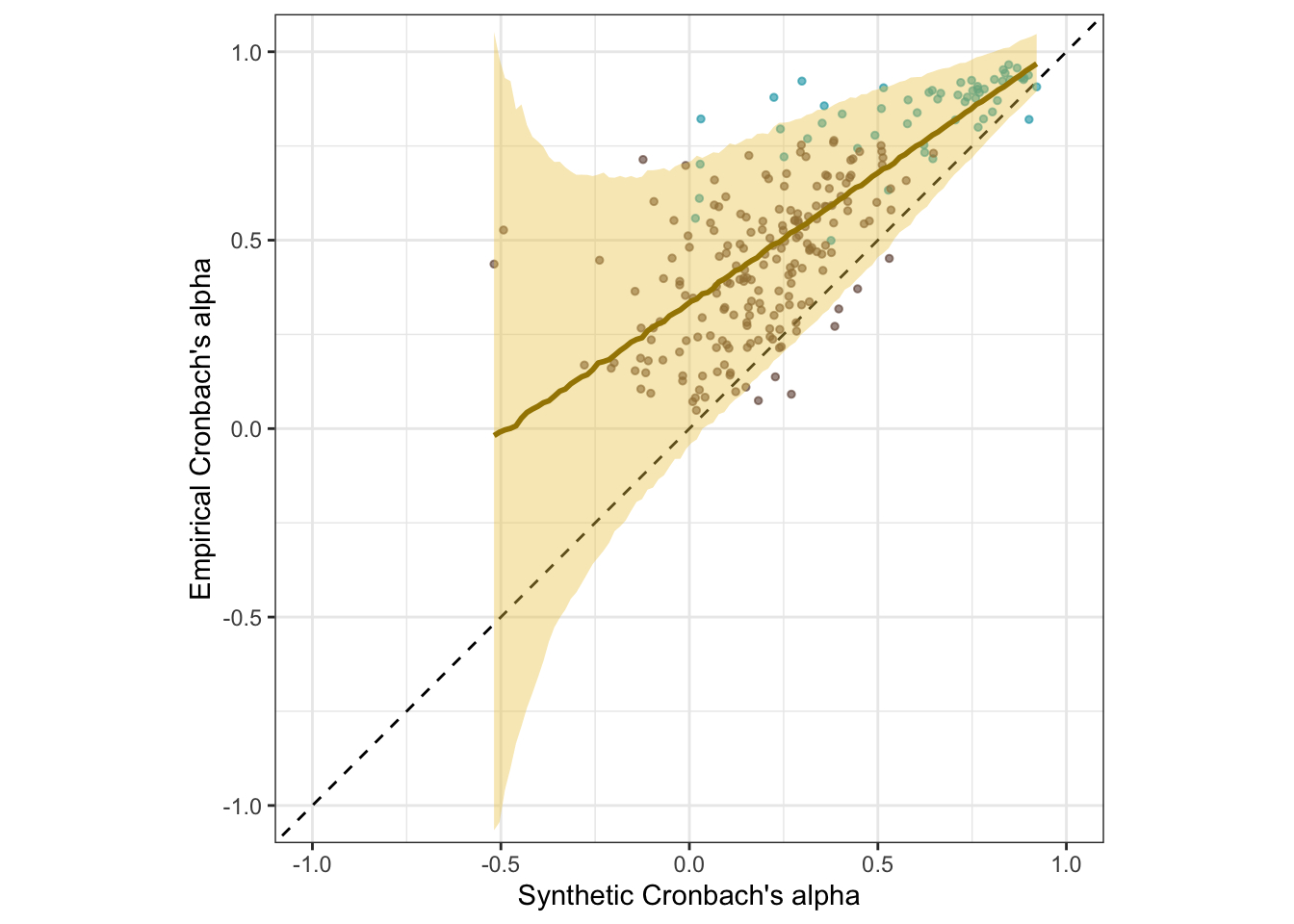

bind_rows(
  r %>% 
    mutate(model = "fine-tuned", kind = "manifest") %>% 
    select(model, kind, accuracy = estimate, conf.low, conf.high),
  s1_r %>% 
    mutate(model = "fine-tuned, conditioned on empirical r", kind = "manifest") %>% 
    select(model, kind, accuracy = estimate, conf.low, conf.high),
  accuracy_bayes_rels %>% 
    mutate(model = "fine-tuned", kind = "latent outcome (Bayesian EIV)") %>% 
    select(model, kind, accuracy = latent_r, conf.low = .lower, conf.high = .upper),
  accuracy_bayes_rels_poly %>% 
    mutate(model = "fine-tuned, conditioned on empirical r", kind = "latent outcome (Bayesian EIV)") %>% 
    select(model, kind, accuracy = latent_r, conf.low = .lower, conf.high = .upper),
  ) %>% 
  knitr::kable(digits = 2, caption = "Accuracy of synthetic alphas when empirical alphas are biased upward through adaptive item reversion and selection on positive alphas")

Accuracy of synthetic alphas when empirical alphas are biased upward through adaptive item reversion and selection on positive alphas

model	kind	accuracy	conf.low	conf.high
fine-tuned	manifest	0.85	0.81	0.88
fine-tuned, conditioned on empirical r	manifest	0.74	0.68	0.80
fine-tuned	latent outcome (Bayesian EIV)	0.84	0.79	0.90
fine-tuned, conditioned on empirical r	latent outcome (Bayesian EIV)	0.77	0.69	0.85

Number of items as a trivial predictor

Although the number of items alone can of course predict Cronbach’s alpha, the synthetic alphas explain much more variance in empirical alphas.

scales %>% 
  ungroup() %>% 
  summarise(broom::tidy(cor.test(number_of_items, empirical_alpha)), sd_alpha = sd(empirical_alpha), n = n()) %>% 
  knitr::kable(digits = 2)

estimate	statistic	p.value	parameter	conf.low	conf.high	method	alternative	sd_alpha	n
0.04	0.67	0.5	255	-0.08	0.16	Pearson’s product-moment correlation	two.sided	0.54	257

summary(lm(empirical_alpha ~ number_of_items, scales))

##
## Call:
## lm(formula = empirical_alpha ~ number_of_items, data = scales)
##
## Residuals:
##     Min      1Q  Median      3Q     Max
## -1.4908 -0.3462 -0.0713  0.3084  0.9129
##
## Coefficients:
##                  Estimate Std. Error t value Pr(>|t|)
## (Intercept)     -0.015196   0.080899  -0.188    0.851
## number_of_items  0.008388   0.012503   0.671    0.503
##
## Residual standard error: 0.5448 on 255 degrees of freedom
## Multiple R-squared:  0.001762,   Adjusted R-squared:  -0.002153
## F-statistic:  0.45 on 1 and 255 DF,  p-value: 0.5029

summary(lm(empirical_alpha ~ number_of_items + synthetic_alpha, scales))

##
## Call:
## lm(formula = empirical_alpha ~ number_of_items + synthetic_alpha,
##     data = scales)
##
## Residuals:
##      Min       1Q   Median       3Q      Max
## -0.94552 -0.14535 -0.01649  0.15466  0.81161
##
## Coefficients:
##                  Estimate Std. Error t value Pr(>|t|)
## (Intercept)     -0.024067   0.043008  -0.560    0.576
## number_of_items -0.002373   0.006660  -0.356    0.722
## synthetic_alpha  1.256941   0.049366  25.462   <2e-16 ***
## ---
## Signif. codes:  0 '***' 0.001 '**' 0.01 '*' 0.05 '.' 0.1 ' ' 1
##
## Residual standard error: 0.2896 on 254 degrees of freedom
## Multiple R-squared:  0.719,  Adjusted R-squared:  0.7168
## F-statistic: 324.9 on 2 and 254 DF,  p-value: < 2.2e-16

Deattenuating accuracy

scales %>% ungroup() %>% 
  summarise(mean(empirical_alpha), sd(empirical_alpha)) %>% 
  kable(digits = 2, caption = "Accuracy across all scales")

Accuracy across all scales

mean(empirical_alpha)	sd(empirical_alpha)
0.03	0.54

scales %>% group_by(type) %>% 
  summarise(mean_alpha = mean(empirical_alpha), 
            sd_alpha = sd(empirical_alpha),
            broom::tidy(cor.test(synthetic_alpha, empirical_alpha)), 
            n = n()) %>% 
  kable(digits = 2, caption = "Accuracy separated by random/real")

Accuracy separated by random/real

type	mean_alpha	sd_alpha	estimate	statistic	p.value	parameter	conf.low	conf.high	method	alternative	n
random	-0.20	0.37	0.63	11.47	0	198	0.54	0.71	Pearson’s product-moment correlation	two.sided	200
real	0.84	0.10	0.64	6.11	0	55	0.45	0.77	Pearson’s product-moment correlation	two.sided	57

psychometric::cRRr(0.647, 0.102, 0.514) %>% 
  kable(digits = 2, caption = "Accuracy for real scales disattenuated for variance restriction")

Accuracy for real scales disattenuated for variance restriction

unrestricted
0.97

Pre-trained model

Is the accuracy lower for the pre-trained model?

ggplot(scales, aes(pt_synthetic_alpha, empirical_alpha, 
                   color = str_detect(scale, "^random"), 
              ymin = empirical_alpha - empirical_alpha_se,
              ymax = empirical_alpha + empirical_alpha_se)) + 
  geom_abline(linetype = "dashed") +
  geom_point(alpha = 0.6, size = 1) +
  scale_color_manual(values = c("#00A0B0", "#6A4A3C"),
                     guide = "none") +
  xlab("Synthetic Cronbach's alpha") + 
  ylab("Empirical Cronbach's alpha") +
  theme_bw() +
  coord_fixed(xlim = c(-1,1), ylim = c(-1,1)) -> pt_plot_rels
pt_plot_rels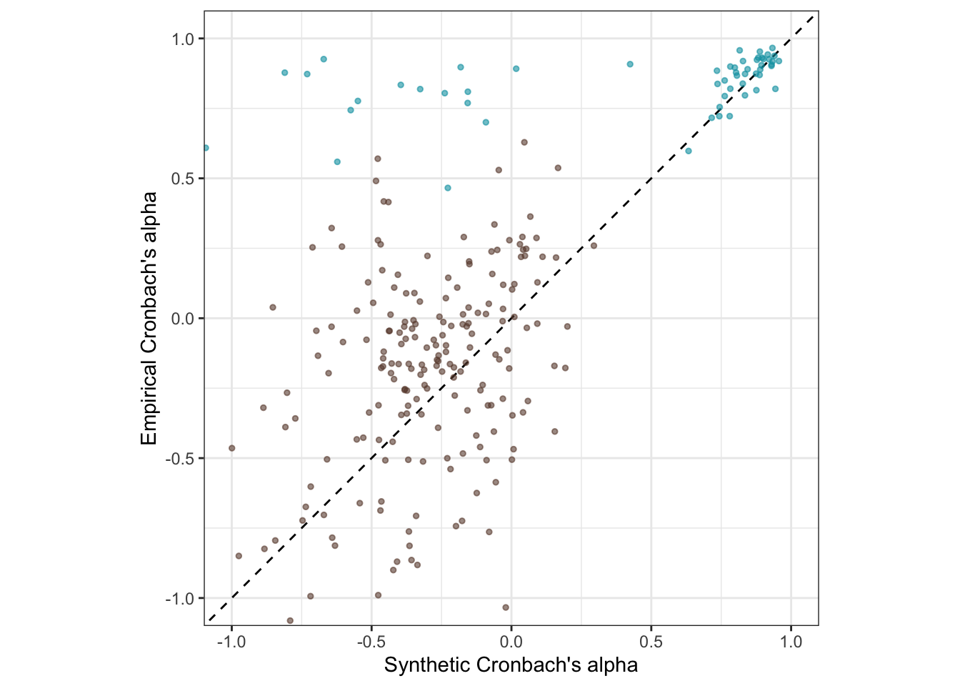

Synthetic Scale Correlations

manifest_scores = arrow::read_feather(file = file.path(data_path, glue("{model_name}.raw.validation-study-2024-11-01.scale_correlations.feather")))
pt_manifest_scores = arrow::read_feather(file = file.path(data_path, glue("{pretrained_model_name}.raw.validation-study-2024-11-01.scale_correlations.feather")))

manifest_scores <- manifest_scores %>%
 left_join(real_scales, by = c("scale_a" = "scale")) %>%
 left_join(real_scales, by = c("scale_b" = "scale")) %>% 
  left_join(pt_manifest_scores %>% select(scale_a, scale_b, pt_synthetic_r = synthetic_r), by = c("scale_a", "scale_b"))

pt_manifest_scores <- pt_manifest_scores %>%
 left_join(real_scales, by = c("scale_a" = "scale")) %>%
 left_join(real_scales, by = c("scale_b" = "scale"))

manifest_scores_all <- manifest_scores
pt_manifest_scores_all <- pt_manifest_scores
manifest_scores <- manifest_scores %>% filter(number_of_items.x >= 3, number_of_items.y >= 3)
pt_manifest_scores <- pt_manifest_scores %>% filter(number_of_items.x >= 3, number_of_items.y >= 3)

Accuracy

r <- broom::tidy(cor.test(manifest_scores$empirical_r, manifest_scores$synthetic_r))
pt_r <- broom::tidy(cor.test(pt_manifest_scores$empirical_r, pt_manifest_scores$synthetic_r))

se2 <- mean(manifest_scores$empirical_r_se^2)
model <- paste0('
    # Latent variables
    PearsonLatent =~ 1*empirical_r

    # Fixing error variances based on known standard errors
    empirical_r ~~ ',se2,'*empirical_r

    # Relationship between latent variables
    PearsonLatent ~~ synthetic_r
  ')

fit <- sem(model, data = manifest_scores)
pt_fit <- sem(model, data = pt_manifest_scores)


pt_m_lmsynth_r_scales <- brm(
  bf(empirical_r | mi(empirical_r_se) ~ synthetic_r + (1|mm(scale_a, scale_b)),
     sigma ~ s(synthetic_r)), data = pt_manifest_scores, 
  file = "ignore/pt_m_synth_rr_r_scales_lm8")

newdata <- pt_m_lmsynth_r_scales$data %>% select(empirical_r, synthetic_r, empirical_r_se)
epreds <- epred_draws(newdata = newdata, obj = pt_m_lmsynth_r_scales, re_formula = NA)
preds <- predicted_draws(newdata = newdata, obj = pt_m_lmsynth_r_scales, re_formula = NA)
epred_preds <- epreds %>% left_join(preds)
by_draw <- epred_preds %>% group_by(.draw) %>% 
  summarise(.epred = var(.epred),
            .prediction = var(.prediction),
            sigma = sqrt(.prediction - .epred),
            latent_r = sqrt(.epred/.prediction))

pt_accuracy_bayes_scales <- by_draw %>% mean_hdci(latent_r)

m_lmsynth_r_scales <- brm(
  bf(empirical_r | mi(empirical_r_se) ~ synthetic_r + (1|mm(scale_a, scale_b)),
     sigma ~ s(synthetic_r)), data = manifest_scores, 
  file = "ignore/m_synth_rr_r_scales_lm8")

sd_synth <- sd(m_lmsynth_r_scales$data$synthetic_r)


newdata <- m_lmsynth_r_scales$data %>% select(empirical_r, synthetic_r, empirical_r_se)
epreds <- epred_draws(newdata = newdata, obj = m_lmsynth_r_scales, re_formula = NA)
preds <- predicted_draws(newdata = newdata, obj = m_lmsynth_r_scales, re_formula = NA)
epred_preds <- epreds %>% left_join(preds)
by_draw <- epred_preds %>% group_by(.draw) %>% 
  summarise(
            mae = mean(abs(.epred - .prediction)),
            .epred = var(.epred),
            .prediction = var(.prediction),
            sigma = sqrt(.prediction - .epred),
            latent_r = sqrt(.epred/.prediction))

accuracy_bayes_scales <- by_draw %>% mean_hdci(latent_r)

bind_rows(
  pt_r %>% 
    mutate(model = "pre-trained", kind = "manifest") %>% 
    select(model, kind, accuracy = estimate, conf.low, conf.high),
  standardizedsolution(pt_fit) %>% 
    filter(lhs == "PearsonLatent", rhs ==  "synthetic_r") %>% 
    mutate(model = "pre-trained", kind = "latent outcome (SEM)") %>% 
    select(model, kind, accuracy = est.std, 
           conf.low = ci.lower, conf.high = ci.upper),
  pt_accuracy_bayes_scales %>% 
    mutate(model = "pre-trained", kind = "latent outcome (Bayesian EIV)") %>% 
    select(model, kind, accuracy = latent_r, conf.low = .lower, conf.high = .upper),
  r %>% 
    mutate(model = "fine-tuned", kind = "manifest") %>% 
    select(model, kind, accuracy = estimate, conf.low, conf.high),
  standardizedsolution(fit) %>% 
    filter(lhs == "PearsonLatent", rhs ==  "synthetic_r") %>% 
    mutate(model = "fine-tuned", kind = "latent outcome (SEM)") %>% 
    select(model, kind, accuracy = est.std, 
           conf.low = ci.lower, conf.high = ci.upper),
  accuracy_bayes_scales %>% 
    mutate(model = "fine-tuned", kind = "latent outcome (Bayesian EIV)") %>% 
    select(model, kind, accuracy = latent_r, conf.low = .lower, conf.high = .upper)
  ) %>% 
  kable(digits = 2, caption = str_c("Accuracy for k=",nrow(manifest_scores)," scale pairs (",n_distinct(c(manifest_scores$scale_a, manifest_scores$scale_b))," scales) across language models and methods"))

Accuracy for k=1568 scale pairs (57 scales) across language models and methods

model	kind	accuracy	conf.low	conf.high
pre-trained	manifest	0.50	0.46	0.54
pre-trained	latent outcome (SEM)	0.51	0.47	0.55
pre-trained	latent outcome (Bayesian EIV)	0.61	0.56	0.66
fine-tuned	manifest	0.83	0.81	0.85
fine-tuned	latent outcome (SEM)	0.84	0.83	0.86
fine-tuned	latent outcome (Bayesian EIV)	0.84	0.82	0.87

Prediction error plot according to synthetic estimate

m_lmsynth_r_scales

##  Family: gaussian
##   Links: mu = identity; sigma = log
## Formula: empirical_r | mi(empirical_r_se) ~ synthetic_r + (1 | mm(scale_a, scale_b))
##          sigma ~ s(synthetic_r)
##    Data: manifest_scores (Number of observations: 1568)
##   Draws: 4 chains, each with iter = 2000; warmup = 1000; thin = 1;
##          total post-warmup draws = 4000
##
## Smooth Terms:
##                           Estimate Est.Error l-95% CI u-95% CI Rhat Bulk_ESS Tail_ESS
## sds(sigma_ssynthetic_r_1)     1.15      0.66     0.17     2.67 1.00      795     1059
##
## Group-Level Effects:
## ~mmscale_ascale_b (Number of levels: 57)
##               Estimate Est.Error l-95% CI u-95% CI Rhat Bulk_ESS Tail_ESS
## sd(Intercept)     0.06      0.01     0.04     0.08 1.00     1294     1706
##
## Population-Level Effects:
##                      Estimate Est.Error l-95% CI u-95% CI Rhat Bulk_ESS Tail_ESS
## Intercept               -0.00      0.01    -0.02     0.02 1.00     1297     2114
## sigma_Intercept         -1.86      0.02    -1.90    -1.82 1.00     3551     2614
## synthetic_r              1.20      0.02     1.16     1.24 1.00     3469     2920
## sigma_ssynthetic_r_1    -1.30      2.28    -6.44     2.16 1.00      989      993
##
## Draws were sampled using sample(hmc). For each parameter, Bulk_ESS
## and Tail_ESS are effective sample size measures, and Rhat is the potential
## scale reduction factor on split chains (at convergence, Rhat = 1).

kable(rmse_scales <- by_draw %>% mean_hdci(sigma), caption = "Average prediction error (RMSE)", digits = 2)

Average prediction error (RMSE)

sigma	.lower	.upper	.width	.point	.interval
0.16	0.14	0.17	0.95	mean	hdci

kable(mae_scales <- by_draw %>% mean_hdci(mae), caption = "Average prediction error (MAE)", digits = 2)

Average prediction error (MAE)

mae	.lower	.upper	.width	.point	.interval
0.13	0.12	0.13	0.95	mean	hdci

plot_prediction_error_scales <- plot(conditional_effects(m_lmsynth_r_scales, dpar = "sigma"), plot = F)[[1]] + 
  theme_bw() + 
  geom_smooth(stat = "identity", color = "#a48500", fill = "#EDC951") + 
  xlab("Synthetic inter-scale correlation") + 
  ylab("Prediction error (sigma)")
plot_prediction_error_scales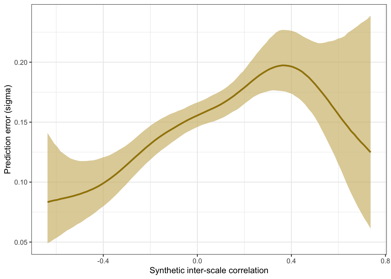

Scatter plot

pred <- conditional_effects(m_lmsynth_r_scales, method = "predict")
ggplot(manifest_scores, aes(synthetic_r, empirical_r, 
              ymin = empirical_r - empirical_r_se,
              ymax = empirical_r + empirical_r_se)) + 
  geom_abline(linetype = "dashed") +
  geom_point(color = "#00A0B0", alpha = 0.1, size = 1) +
  geom_smooth(aes(
    x = synthetic_r,
    y = estimate__,
    ymin = lower__,
    ymax = upper__,
  ), stat = "identity", 
  color = "#a48500",
  fill = "#EDC951",
  data = as.data.frame(pred$synthetic_r)) +
  xlab("Synthetic inter-scale correlation") + 
  ylab("Empirical inter-scale correlation") +
  theme_bw() +
  coord_fixed(xlim = c(-1,1), ylim = c(-1,1)) -> plot_scales
plot_scales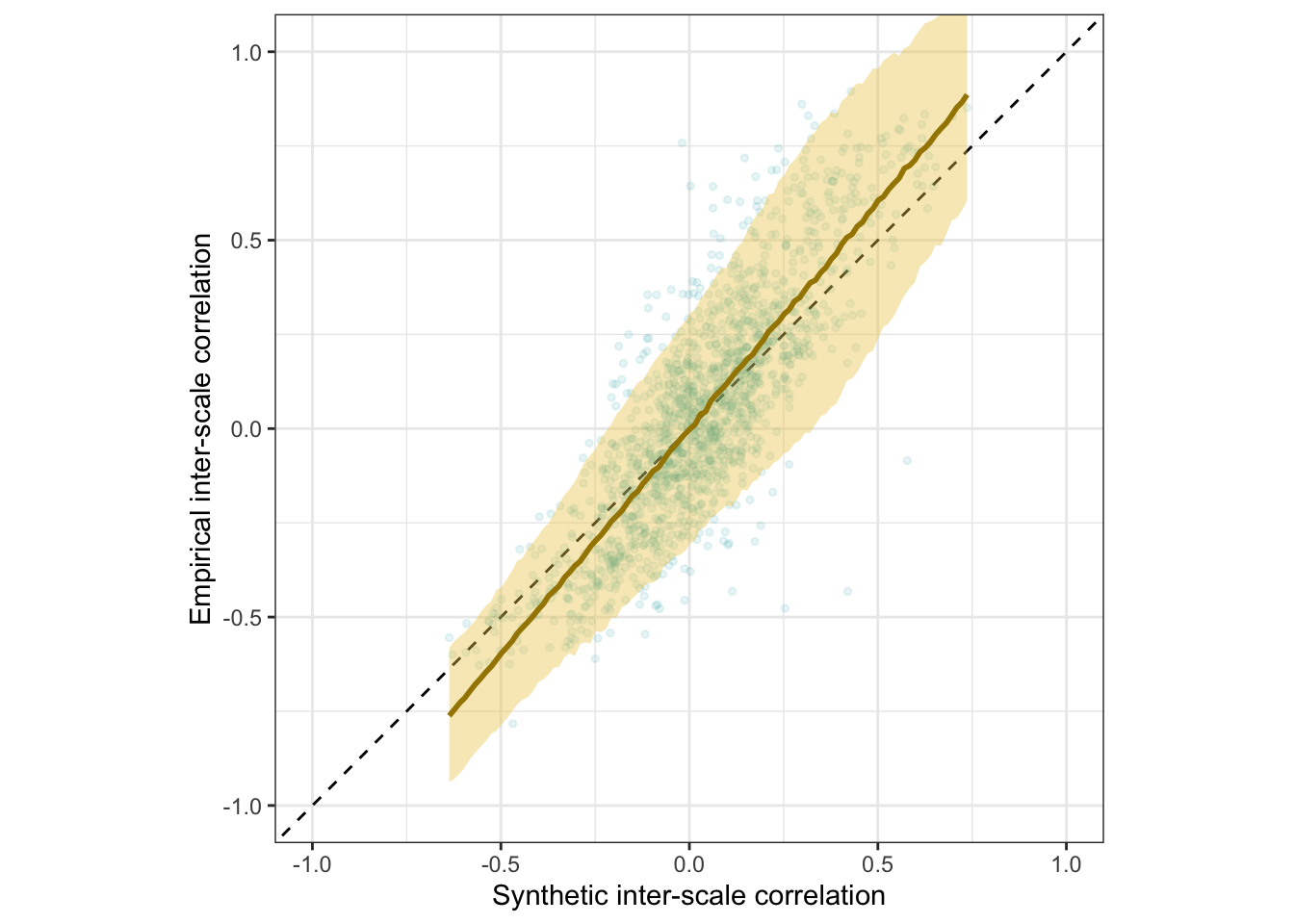

Interactive plot

(manifest_scores %>% 
  mutate(synthetic_r = round(synthetic_r, 2),
         empirical_r = round(empirical_r, 2),
         scales = str_replace_all(str_c(scale_a, "\n", scale_b),
                                  "_+", " ")) %>% 
ggplot(., aes(synthetic_r, empirical_r, 
              # ymin = empirical_r - empirical_r_se, 
              # ymax = empirical_r + empirical_r_se, 
              label = scales)) + 
  geom_abline(linetype = "dashed") +
  geom_point(color = "#00A0B0", alpha = 0.3, size = 1) +
  xlab("Synthetic inter-scale correlation") + 
  ylab("Empirical inter-scale correlation") +
  theme_bw() +
  coord_fixed(xlim = c(-1,1), ylim = c(-1,1))) %>% 
  ggplotly()

Table

manifest_scores %>% 
                mutate(empirical_r = sprintf("%.2f±%.3f", empirical_r,
                                             empirical_r_se),
                       synthetic_r = sprintf("%.2f", synthetic_r),
                       scale_a = str_replace_all(scale_a, "_+", " "),
                       scale_b = str_replace_all(scale_b, "_+", " ")
                       ) %>% 
                select(scale_a, scale_b, empirical_r, synthetic_r) %>% 
  DT::datatable(rownames = FALSE,
                filter = "top")

Robustness checks

Comparing spline and polynomial models for heteroscedasticity

# For scale correlations
m_lmsynth_r_scales_poly <- brm(
  bf(empirical_r | mi(empirical_r_se) ~ synthetic_r + (1|mm(scale_a, scale_b)),
     sigma ~ poly(synthetic_r, degree = 3)), data = manifest_scores, 
  file = "ignore/m_synth_rr_r_scales_lm_poly")

newdata <- m_lmsynth_r_scales_poly$data %>% select(empirical_r, synthetic_r, empirical_r_se)
epreds <- epred_draws(newdata = newdata, obj = m_lmsynth_r_scales_poly, re_formula = NA)
preds <- predicted_draws(newdata = newdata, obj = m_lmsynth_r_scales_poly, re_formula = NA)
epred_preds <- epreds %>% left_join(preds)
by_draw <- epred_preds %>% group_by(.draw) %>% 
  summarise(.epred = var(.epred),
            .prediction = var(.prediction),
            sigma = sqrt(.prediction - .epred),
            latent_r = sqrt(.epred/.prediction))

accuracy_bayes_scales_poly <- by_draw %>% mean_hdci(latent_r)

bind_rows(
  accuracy_bayes_scales %>% 
    mutate(model = "spline", kind = "latent outcome (Bayesian EIV)") %>% 
    select(model, kind, accuracy = latent_r, conf.low = .lower, conf.high = .upper),
  accuracy_bayes_scales_poly %>% 
    mutate(model = "polynomial", kind = "latent outcome (Bayesian EIV)") %>% 
    select(model, kind, accuracy = latent_r, conf.low = .lower, conf.high = .upper)
) %>% 
  knitr::kable(digits = 2, caption = "Comparing spline and polynomial models for scale correlations")

Comparing spline and polynomial models for scale correlations

model	kind	accuracy	conf.low	conf.high
spline	latent outcome (Bayesian EIV)	0.84	0.82	0.87
polynomial	latent outcome (Bayesian EIV)	0.85	0.82	0.87

plot_prediction_error_scales_poly <- plot(conditional_effects(m_lmsynth_r_scales_poly, dpar = "sigma"), plot = F)[[1]] + 
  theme_bw() + 
  geom_smooth(stat = "identity", color = "#a48500", fill = "#EDC951") + 
  xlab("Synthetic inter-scale correlation") + 
  ylab("Prediction error (sigma)")
plot_prediction_error_scales_poly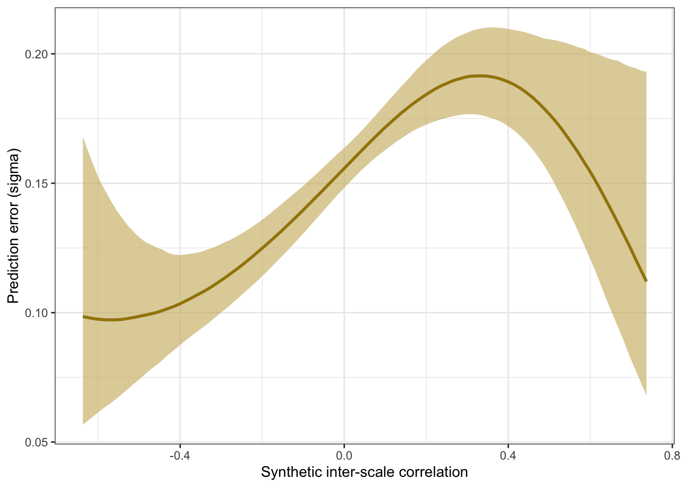

How does number of items across the two scales relate to accuracy?

by_item_number <- manifest_scores_all %>%
  mutate(items = number_of_items.x + number_of_items.y) %>%
  group_by(items) %>%
  filter(n() > 10) %>% 
  summarise(broom::tidy(cor.test(empirical_r, synthetic_r)), pt_cor = cor(empirical_r, pt_synthetic_r), pairwise_n = n()) 

by_item_number %>% 
  ggplot(aes(items, estimate, ymin = conf.low, ymax = conf.high)) + 
  geom_pointrange() +
  scale_y_continuous("Manifest accuracy (with 95% confidence interval)") +
  xlab("Number of items summed across scales")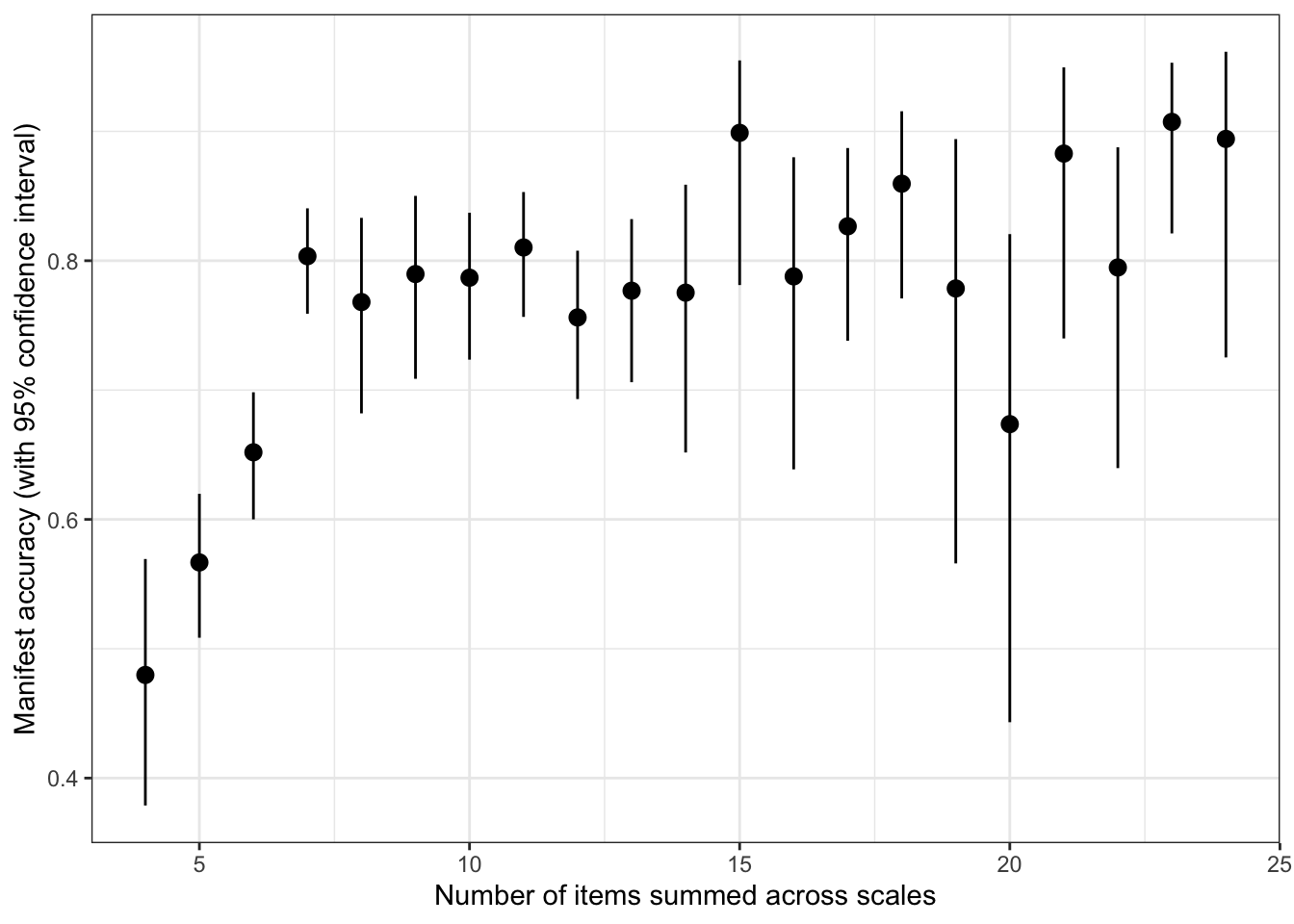

Averages

real_scales %>% ungroup() %>% 
  filter(number_of_items >= 3) %>% 
  summarise(median(number_of_items),
            mean(number_of_items))

## # A tibble: 1 × 2
##   `median(number_of_items)` `mean(number_of_items)`
##                       <int>                   <dbl>
## 1                         4                    5.75

Accuracy including 2-item scales

r_2item <- broom::tidy(cor.test(manifest_scores_all$empirical_r, manifest_scores_all$synthetic_r))
pt_r_2item <- broom::tidy(cor.test(pt_manifest_scores_all$empirical_r, pt_manifest_scores_all$synthetic_r))

bind_rows(
  pt_r %>% 
    mutate(model = "pre-trained", kind = "manifest") %>% 
    select(model, kind, accuracy = estimate, conf.low, conf.high) %>% 
    mutate(items = ">= 3"),
  r %>% 
    mutate(model = "fine-tuned", kind = "manifest") %>% 
    select(model, kind, accuracy = estimate, conf.low, conf.high) %>% 
    mutate(items = ">= 3"),
  pt_r_2item %>% 
    mutate(model = "pre-trained", kind = "manifest") %>% 
    select(model, kind, accuracy = estimate, conf.low, conf.high) %>% 
    mutate(items = ">= 2"),
  r_2item %>% 
    mutate(model = "fine-tuned", kind = "manifest") %>% 
    select(model, kind, accuracy = estimate, conf.low, conf.high) %>% 
    mutate(items = ">= 2"),
  ) %>% 
  kable(digits = 2, caption = "Accuracy across language models and methods")

Accuracy across language models and methods

model	kind	accuracy	conf.low	conf.high	items
pre-trained	manifest	0.50	0.46	0.54	>= 3
fine-tuned	manifest	0.83	0.81	0.85	>= 3
pre-trained	manifest	0.47	0.44	0.49	>= 2
fine-tuned	manifest	0.75	0.73	0.76	>= 2

broom::tidy(lm(estimate ~ items, by_item_number, weights = 1/(by_item_number$conf.high-by_item_number$conf.low))) %>% 
  kable(digits = 2, caption = "Accuracy increase with number of items")

Accuracy increase with number of items

term	estimate	std.error	statistic	p.value
(Intercept)	0.62	0.04	15.62	0
items	0.01	0.00	4.29	0

manifest_scores %>%
  filter(number_of_items.x >= 5, number_of_items.y >= 5) %>%
  summarise(cor = cor(empirical_r, synthetic_r), n()) %>% 
  kable(digits = 2, caption = "Accuracy when both scales have at least 5 items")

Accuracy when both scales have at least 5 items

cor	n()
0.88	228

manifest_scores %>%
  filter(number_of_items.x >= 10, number_of_items.y >= 10) %>%
  summarise(cor = cor(empirical_r, synthetic_r), n()) %>% 
  kable(digits = 2, caption = "Accuracy when both scales have at least 10 items")

Accuracy when both scales have at least 10 items

cor	n()
0.87	36

Is the accuracy lower for the pre-trained model?

ggplot(pt_manifest_scores, aes(synthetic_r, empirical_r, 
              ymin = empirical_r - empirical_r_se,
              ymax = empirical_r + empirical_r_se)) + 
  geom_abline(linetype = "dashed") +
  geom_point(color = "#00A0B0", alpha = 0.1, size = 1) +
  xlab("Synthetic inter-scale correlation") + 
  ylab("Empirical inter-scale correlation") +
  theme_bw() +
  coord_fixed(xlim = c(-1,1), ylim = c(-1,1)) -> pt_plot_scales
pt_plot_scales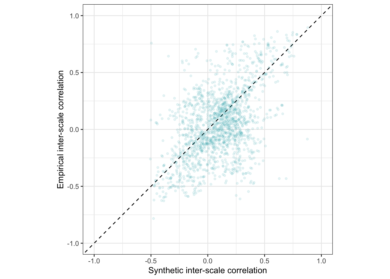

Combined plots

Accuracy scatterplots

library(patchwork)
pt_plot_items2 <- pt_plot_items +
  annotate("text", size = 3, x = -1, y = 0.98, vjust = 0, hjust = 0, label = with(pt_accuracy_bayes_items, { sprintf("accuracy = %.2f [%.2f;%.2f]", latent_r, .lower, .upper) })) +
  annotate("text", size = 2.5, x = -.1, y = 0.5, vjust = 1, hjust = 1, label = "r(CESD_10,19)", color = "#00A0B0") +
  annotate("segment", x = -.1, y = 0.5, xend = 0.4185763, yend = 0.5875796, color = "#00A0B0", alpha = 0.7) +
  
  annotate("text", size = 2.5, x = 0, y = -0.9, hjust = 0.5, label = "r(RAAS_02,05)", color = "#00A0B0") + 
  annotate("segment", x = 0, y = -0.83, xend = 0.5842606, yend = -0.7020895, color = "#00A0B0", alpha = 0.7)
  
plot_items2 <- plot_items +
  annotate("text", size = 3, x = -1, y = 0.98, vjust = 0, hjust = 0, label = with(accuracy_bayes_items, { sprintf("accuracy = %.2f [%.2f;%.2f]", latent_r, .lower, .upper) })) +
  annotate("text", size = 2.5, x = -.1, y = 0.5, vjust = 1, hjust = 1, label = "r(CESD_10,19)", color = "#00A0B0") +
  annotate("segment", x = -.1, y = 0.5, xend = 0.5369071, yend = 0.5875796, color = "#00A0B0", alpha = 0.7) +
  
  annotate("text", size = 2.5, x = 0, y = -0.9, hjust = 0.5, label = "r(RAAS_02,05)", color = "#00A0B0") + 
  annotate("segment", x = 0, y = -0.83, xend = 0.09218573, yend = -0.7020895, color = "#00A0B0", alpha = 0.7)

pt_plot_rels2 <- pt_plot_rels + 
  annotate("text", size = 3, x = -1, y = .98, vjust = 0, hjust = 0, label = with(pt_accuracy_bayes_rels, { sprintf("accuracy = %.2f [%.2f;%.2f]", latent_r, .lower, .upper) })) +
  annotate("text", size = 2.5,  x = 0.68, y = 0, hjust = 0.5, label = "Fear of COVID", color = "#00A0B0") +
  annotate("segment",  x = 0.68, y = 0.05, xend = 0.9563192, yend = 0.9262542, color = "#00A0B0", alpha = 0.7) +
  
  annotate("text", size = 2.5, x = -1, y = 0.5, hjust = 0, label = "HEXACO fairness", color = "#00A0B0") +
  annotate("segment", x = -0.65, y = 0.55,  xend = -0.3262759, yend = 0.8217475, color = "#00A0B0", alpha = 0.7)


get_scale_point <- function(data, synthetic_approx, empirical_approx) {
  data %>%
    ungroup() %>% 
    # Find closest point to target coordinates
    mutate(dist = sqrt((synthetic_alpha - synthetic_approx)^2 + 
                      (empirical_alpha - empirical_approx)^2)) %>%
    arrange(dist) %>%
    slice(1) %>%
    select(synthetic_alpha, empirical_alpha)
}
p1 <- get_scale_point(scales, 0.30, 0.22)
p2 <- get_scale_point(scales, 0.12, -0.36) 
p3 <- get_scale_point(scales, -0.4, -0.90)

plot_rels2 <- plot_rels + 
  annotate("text", size = 3, x = -1, y = .98, vjust = 0, hjust = 0, label = with(accuracy_bayes_rels, { sprintf("accuracy = %.2f [%.2f;%.2f]", latent_r, .lower, .upper) })) +
  annotate("text", size = 2.5, x = -0.2, y = -0.9, hjust = 0, label = "randomly formed scales", color = "#6A4A3C") +
  annotate("segment", x = 0.4, y = -0.85, xend = p1$synthetic_alpha, yend = p1$empirical_alpha, color = "#6A4A3C", alpha = 0.7) +
  annotate("segment", x = 0.4, y = -0.85, xend = p2$synthetic_alpha, yend = p2$empirical_alpha, color = "#6A4A3C", alpha = 0.7) +
  annotate("segment", x = 0.4, y = -0.85, xend = p3$synthetic_alpha, yend = p3$empirical_alpha, color = "#6A4A3C", alpha = 0.7) +
  
  annotate("text", size = 2.5, x = 0.68, y = 0, hjust = 0.5, label = "Fear of COVID", color = "#00A0B0") +
  annotate("segment", x = 0.68, y = 0.05, xend = 0.8864024, yend = 0.9262542, color = "#00A0B0", alpha = 0.7) +
  
  annotate("text", size = 2.5, x = -1, y = 0.5, hjust = 0,label = "HEXACO fairness", color = "#00A0B0") +
  annotate("segment", x = -0.65, y = 0.55, xend = 0.0305553, yend = 0.8217475, color = "#00A0B0", alpha = 0.7)


pt_plot_scales2 <- pt_plot_scales +
  annotate("text", size = 3, x = -1, y = 0.98, vjust = 0, hjust = 0, label = with(pt_accuracy_bayes_scales, { sprintf("accuracy = %.2f [%.2f;%.2f]", latent_r, .lower, .upper) })) +
  annotate("text", size = 2.5, x = -0.4, y = 0.5, hjust = 1, label = "r(UWES vigor,\nWGS)", color = "#00A0B0") +
  annotate("segment", x = -.38, y = 0.45, xend = 0.6586402, yend = 0.5683167, color = "#00A0B0", alpha = 0.7) +
  
  annotate("text", size = 2.5, x = -.1, y = -0.9, hjust = 0.5, label = "r(CES-D well-being,\nCES-D depressive affect)", color = "#00A0B0") +
  annotate("segment", x = -0.2, y = -.75, xend = 0.4963392, yend = -0.7583637, color = "#00A0B0", alpha = 0.7)


plot_scales2 <- plot_scales +
  annotate("text", size = 3, x = -1, y = 0.98, vjust = 0, hjust = 0, label = with(accuracy_bayes_scales, { sprintf("accuracy = %.2f [%.2f;%.2f]", latent_r, .lower, .upper) })) +
  annotate("text", size = 2.5, x = -0.4, y = 0.5, hjust = 1, label = "r(UWES vigor,\nWGS)", color = "#00A0B0") +
  annotate("segment", x = -.38, y = 0.45, xend = .55, yend = 0.5683167, color = "#00A0B0", alpha = 0.7) +
  
  annotate("text", size = 2.5, x = -.1, y = -0.9, hjust = 0.5, label = "r(CES-D well-being,\nCES-D depressive affect)", color = "#00A0B0") +
  annotate("segment", x = -0.2, y = -.75, xend = 0.02, yend = -0.7583637, color = "#00A0B0", alpha = 0.7)


(pt_plot_items2 + ggtitle("Pre-trained model before domain adaptation and fine-tuning") +
    pt_plot_rels2 +
    pt_plot_scales2) /


(plot_items2 + ggtitle("SurveyBot 3000") +
    plot_rels2  +
    plot_scales2)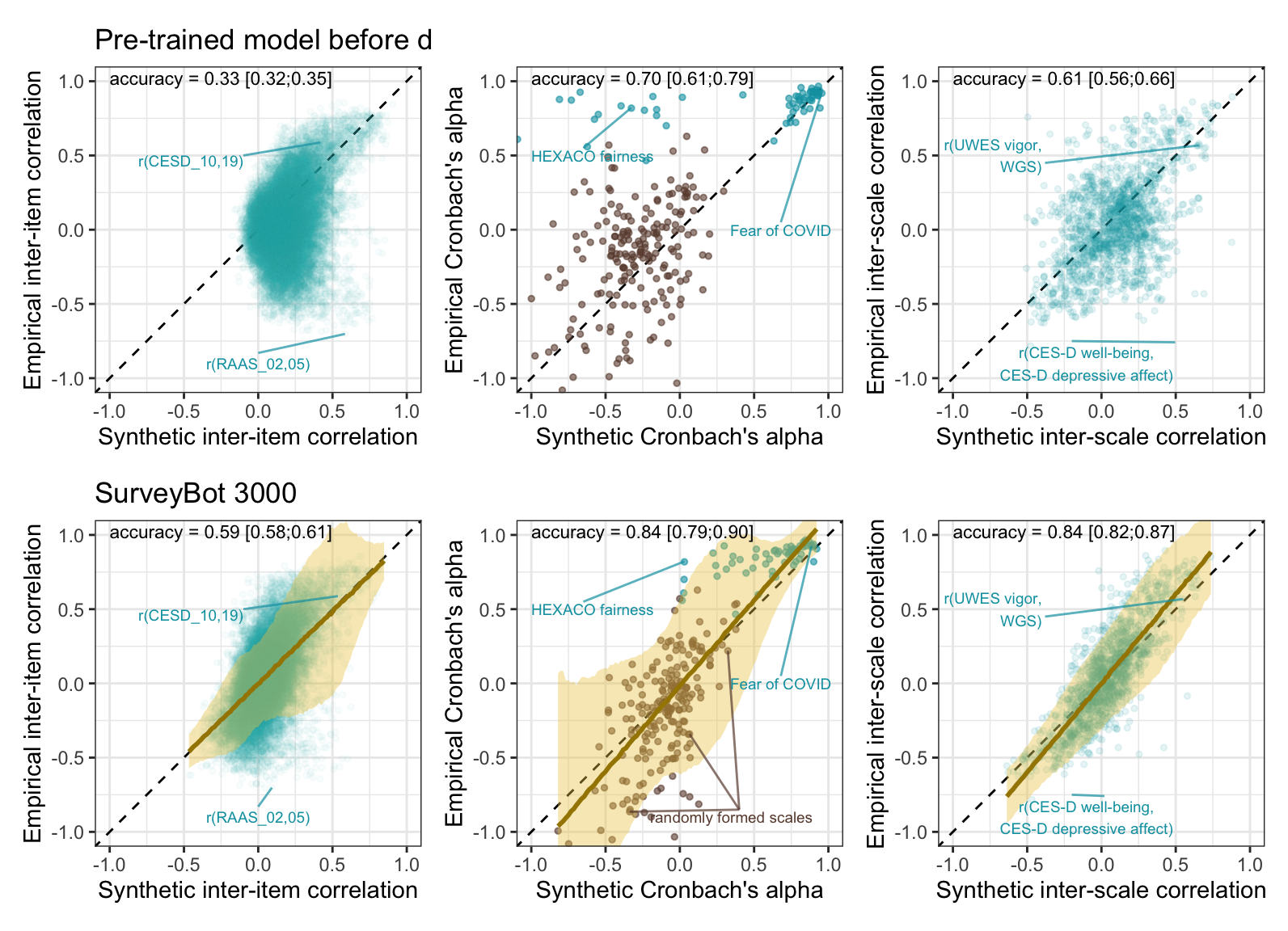

ggsave("Figure_rr.pdf", width = 8.3, height = 6, device = grDevices::cairo_pdf)
ggsave("Figure_rr.png", width = 8.3, height = 6)

Prediction error plots

library(patchwork)

(plot_prediction_error_items + 
    coord_cartesian(xlim = c(-1, 1), ylim = c(0, 0.4)) +
    annotate("text", size = 3, x = -1, y = 0.4, vjust = 0, hjust = 0, label = with(rmse_items, { sprintf("RMSE = %.2f [%.2f;%.2f]", sigma, .lower, .upper) })) +
    
    plot_prediction_error_alpha + 
    coord_cartesian(xlim = c(-1, 1), ylim = c(0, 0.4))  +
    annotate("text", size = 3, x = -1, y = 0.4, vjust = 0, hjust = 0, label = with(rmse_alpha, { sprintf("RMSE = %.2f [%.2f;%.2f]", sigma, .lower, .upper) })) +
    
    plot_prediction_error_scales + 
    coord_cartesian(xlim = c(-1, 1), ylim = c(0, 0.4)) +
    annotate("text", size = 3, x = -1, y = 0.4, vjust = 0, hjust = 0, label = with(rmse_scales, { sprintf("RMSE = %.2f [%.2f;%.2f]", sigma, .lower, .upper) }))
)

ggsave("ignore/Figure_prediction_error_rr.pdf", width = 8.3, height = 3, device = grDevices::cairo_pdf)
ggsave("ignore/Figure_prediction_error_rr.png", width = 8.3, height = 3)